Tidy Transcriptomics for Single-cell RNA Sequencing Analyses

Instructors

Dr. Stefano Mangiola is currently a Postdoctoral researcher in the laboratory of Prof. Tony Papenfuss at the Walter and Eliza Hall Institute in Melbourne, Australia. His background spans from biotechnology to bioinformatics and biostatistics. His research focuses on prostate and breast tumour microenvironment, the development of statistical models for the analysis of RNA sequencing data, and data analysis and visualisation interfaces.

Dr. Maria Doyle is the Application and Training Specialist for Research Computing at the Peter MacCallum Cancer Centre in Melbourne, Australia. She has a PhD in Molecular Biology and currently works in bioinformatics and data science education and training. She is passionate about supporting researchers, reproducible research, open source and tidy data.

Workshop goals and objectives

What you will learn

Basic tidy operations possible with tidyseurat and tidySingleCellExperiment
The differences between Seurat and SingleCellExperiment representation, and tidy representation
How to interface Seurat and SingleCellExperiment with tidy manipulation and visualisation
A real-world case study that will showcase the power of tidy single-cell methods compared with base/ad-hoc methods

What you will not learn

The molecular technology of single-cell sequencing
The fundamentals of single-cell data analysis
The fundamentals of tidy data analysis

Slides

Getting started

Cloud

Easiest way to run this material. Only available during workshop. Many thanks to the Australian Research Data Commons (ARDC) for providing RStudio in the Australian Nectar Research Cloud and Andy Botting from ARDC for helping to set up.

Login to one of the servers (e.g. https://rstudio5.tidytranscriptomics-workshop.cloud.edu.au/rstudio/) with one of the usernames and passwords from the spreadsheet provided at the workshop. Add your name into the spreadsheet beside the login you’re using.
Open tidytranscriptomics_case_study.Rmd in iscb2022_tidytranscriptomcs/vignettes folder

Local

We will use the Cloud during the ISCB workshop and this method is available if you want to run the material after the workshop. If you want to install on your own computer, see instructions here.

Alternatively, you can view the material at the workshop webpage here.

library(Seurat)
library(ggplot2)
library(plotly)
library(dplyr)
library(colorspace)
library(SeuratWrappers)
library(dittoSeq)

Introduction to tidyseurat

Seurat is a very popular analysis toolkit for single cell RNA sequencing data (Butler et al. 2018; Stuart et al. 2019).

Here we load single-cell data in Seurat object format. This data is peripheral blood mononuclear cells (PBMCs) from metastatic breast cancer patients.

# load single cell RNA sequencing data
seurat_obj <- iscb2022tidytranscriptomics::seurat_obj

# take a look
seurat_obj

## An object of class Seurat 
## 3006 features across 36683 samples within 2 assays 
## Active assay: SCT (6 features, 0 variable features)
##  1 other assay present: RNA
##  1 dimensional reduction calculated: umap

tidyseurat provides a bridge between the Seurat single-cell package and the tidyverse (Wickham et al. 2019). It creates an invisible layer that enables viewing the Seurat object as a tidyverse tibble, and provides Seurat-compatible dplyr, tidyr, ggplot and plotly functions.

If we load the tidyseurat package and then view the single cell data, it now displays as a tibble.

library(tidyseurat)

seurat_obj

## # A Seurat-tibble abstraction: 36,683 × 15
## # Features=6 | Active assay=SCT | Assays=RNA, SCT
##    .cell file  Barcode batch BCB    S.Score G2M.Score Phase curated_cell_ty…
##    <chr> <chr> <chr>   <chr> <chr>    <dbl>     <dbl> <chr> <chr>           
##  1 1_AA… ../d… AAACCC… 1     BCB1… -0.00277   -0.103  G1    CD4+_ribosome_r…
##  2 1_AA… ../d… AAACGA… 1     BCB1…  0.0620    -0.0972 S     CD4+_Tcm_S100A4…
##  3 1_AA… ../d… AAACGC… 1     BCB1…  0.0943    -0.193  S     CD8+_high_ribon…
##  4 1_AA… ../d… AAACGC… 1     BCB1… -0.0676    -0.205  G1    CD4+_ribosome_r…
##  5 1_AA… ../d… AAACGC… 1     BCB1…  0.0216    -0.124  S     CD4+_Tcm_S100A4…
##  6 1_AA… ../d… AAAGAA… 1     BCB1…  0.0598    -0.196  S     MAIT            
##  7 1_AA… ../d… AAAGGA… 1     BCB1…  0.0281    -0.0540 S     CD8+_high_ribon…
##  8 1_AA… ../d… AAAGGG… 1     BCB1…  0.0110    -0.0998 S     MAIT            
##  9 1_AA… ../d… AAAGGG… 1     BCB1…  0.0341    -0.143  S     CD8+_high_ribon…
## 10 1_AA… ../d… AAAGTC… 1     BCB1…  0.0425    -0.183  S     MAIT            
## # … with 36,673 more rows, and 6 more variables: nCount_RNA <dbl>,
## #   nFeature_RNA <int>, nCount_SCT <dbl>, nFeature_SCT <int>, UMAP_1 <dbl>,
## #   UMAP_2 <dbl>

It can be interacted with using Seurat commands such as Assays.

Assays(seurat_obj)

## [1] "RNA" "SCT"

We can also interact with our object as we do with any tidyverse tibble.

Tidyverse commands

We can use tidyverse commands, such as filter, select and mutate to explore the tidyseurat object. Some examples are shown below and more can be seen at the tidyseurat website here.

We can use filter to choose rows, for example, to see just the rows for the cells in G1 cell-cycle stage. Check if have groups or ident present.

seurat_obj |> filter(Phase == "G1")

## # A Seurat-tibble abstraction: 19,968 × 15
## # Features=6 | Active assay=SCT | Assays=RNA, SCT
##    .cell file  Barcode batch BCB    S.Score G2M.Score Phase curated_cell_ty…
##    <chr> <chr> <chr>   <chr> <chr>    <dbl>     <dbl> <chr> <chr>           
##  1 1_AA… ../d… AAACCC… 1     BCB1… -0.00277  -0.103   G1    CD4+_ribosome_r…
##  2 1_AA… ../d… AAACGC… 1     BCB1… -0.0676   -0.205   G1    CD4+_ribosome_r…
##  3 1_AA… ../d… AAAGTC… 1     BCB1… -0.0289   -0.127   G1    CD8+_high_ribon…
##  4 1_AA… ../d… AAAGTG… 1     BCB1… -0.0551   -0.102   G1    CD8+_high_ribon…
##  5 1_AA… ../d… AAATGG… 1     BCB1… -0.0207   -0.0602  G1    TCR_V_Delta_2   
##  6 1_AA… ../d… AAATGG… 1     BCB1… -0.0195   -0.00881 G1    CD4+_Tcm_S100A4…
##  7 1_AA… ../d… AACAAC… 1     BCB1… -0.0421   -0.197   G1    CD4+_Tcm_S100A4…
##  8 1_AA… ../d… AACAAC… 1     BCB1… -0.0105   -0.0902  G1    CD4+_Tcm_S100A4…
##  9 1_AA… ../d… AACACA… 1     BCB1… -0.0164   -0.132   G1    MAIT            
## 10 1_AA… ../d… AACAGG… 1     BCB1… -0.00158  -0.0652  G1    NK_cells        
## # … with 19,958 more rows, and 6 more variables: nCount_RNA <dbl>,
## #   nFeature_RNA <int>, nCount_SCT <dbl>, nFeature_SCT <int>, UMAP_1 <dbl>,
## #   UMAP_2 <dbl>

We can use select to choose columns, for example, to see the sample, cell, total cellular RNA

seurat_obj |> select(.cell, nCount_RNA, Phase)

## # A Seurat-tibble abstraction: 36,683 × 5
## # Features=6 | Active assay=SCT | Assays=RNA, SCT
##    .cell                nCount_RNA Phase  UMAP_1 UMAP_2
##    <chr>                     <dbl> <chr>   <dbl>  <dbl>
##  1 1_AAACCCACACGACGCT-1       1673 G1    -1.23   -2.95 
##  2 1_AAACGAACAAAGGCAC-1       1485 S      2.56   -2.99 
##  3 1_AAACGCTCATGAATAG-1       2460 S     -3.32   -3.84 
##  4 1_AAACGCTTCATTCATC-1       1937 G1    -0.0650 -3.16 
##  5 1_AAACGCTTCTTGGATG-1       1739 S      2.51   -3.15 
##  6 1_AAAGAACCAACGGCTC-1       2346 S     -3.11   -0.166
##  7 1_AAAGGATTCCCGTTCA-1        763 S     -3.50   -0.754
##  8 1_AAAGGGCAGGCATTTC-1       2001 S      1.54   -2.10 
##  9 1_AAAGGGCCAGAGATTA-1       1907 S     -3.20   -1.92 
## 10 1_AAAGTCCAGTAACGAT-1       2239 S     -4.03    0.347
## # … with 36,673 more rows

We also see the UMAP columns as they are not part of the cell metadata, they are read-only. If we want to save the edited metadata, the Seurat object is modified accordingly.

# Save edited metadata
seurat_modified <- seurat_obj |> select(.cell, nCount_RNA, Phase)
# View Seurat metadata
seurat_modified[[]] |> head()

##                      nCount_RNA Phase
## 1_AAACCCACACGACGCT-1       1673    G1
## 1_AAACGAACAAAGGCAC-1       1485     S
## 1_AAACGCTCATGAATAG-1       2460     S
## 1_AAACGCTTCATTCATC-1       1937    G1
## 1_AAACGCTTCTTGGATG-1       1739     S
## 1_AAAGAACCAACGGCTC-1       2346     S

We can use mutate to create a column. For example, we could create a new Phase_l column that contains a lower-case version of Phase.

seurat_obj |>
  mutate(Phase_l=tolower(Phase)) |>
  
  # Select columns to view    
  select(Phase, Phase_l)

## tidyseurat says: Key columns are missing. A data frame is returned for independent data analysis.

## # A tibble: 36,683 × 2
##    Phase Phase_l
##    <chr> <chr>  
##  1 G1    g1     
##  2 S     s      
##  3 S     s      
##  4 G1    g1     
##  5 S     s      
##  6 S     s      
##  7 S     s      
##  8 S     s      
##  9 S     s      
## 10 S     s      
## # … with 36,673 more rows

We can use tidyverse commands to polish an annotation column. We will extract the sample, and group information from the file name column into separate columns.

# First take a look at the file column
seurat_obj |> select(file)

## tidyseurat says: Key columns are missing. A data frame is returned for independent data analysis.

## # A tibble: 36,683 × 1
##    file                                                              
##    <chr>                                                             
##  1 ../data/experiment_10X_260819/SI-GA-H1/outs/raw_feature_bc_matrix/
##  2 ../data/experiment_10X_260819/SI-GA-H1/outs/raw_feature_bc_matrix/
##  3 ../data/experiment_10X_260819/SI-GA-H1/outs/raw_feature_bc_matrix/
##  4 ../data/experiment_10X_260819/SI-GA-H1/outs/raw_feature_bc_matrix/
##  5 ../data/experiment_10X_260819/SI-GA-H1/outs/raw_feature_bc_matrix/
##  6 ../data/experiment_10X_260819/SI-GA-H1/outs/raw_feature_bc_matrix/
##  7 ../data/experiment_10X_260819/SI-GA-H1/outs/raw_feature_bc_matrix/
##  8 ../data/experiment_10X_260819/SI-GA-H1/outs/raw_feature_bc_matrix/
##  9 ../data/experiment_10X_260819/SI-GA-H1/outs/raw_feature_bc_matrix/
## 10 ../data/experiment_10X_260819/SI-GA-H1/outs/raw_feature_bc_matrix/
## # … with 36,673 more rows

# Create columns for sample and group
seurat_obj <- seurat_obj |>

# Extract sample and group
  extract(file, "sample", "../data/.*/([a-zA-Z0-9_-]+)/outs.+", remove = FALSE)

# Take a look
seurat_obj |> select(sample)

## tidyseurat says: Key columns are missing. A data frame is returned for independent data analysis.

## # A tibble: 36,683 × 1
##    sample  
##    <chr>   
##  1 SI-GA-H1
##  2 SI-GA-H1
##  3 SI-GA-H1
##  4 SI-GA-H1
##  5 SI-GA-H1
##  6 SI-GA-H1
##  7 SI-GA-H1
##  8 SI-GA-H1
##  9 SI-GA-H1
## 10 SI-GA-H1
## # … with 36,673 more rows

We could use tidyverse unite to combine columns, for example to create a new column for sample id that combines the sample and patient identifier (BCB) columns.

seurat_obj <- seurat_obj |> unite("sample_id", sample, BCB, remove = FALSE)

# Take a look
seurat_obj |> select(sample_id, sample, BCB)

## tidyseurat says: Key columns are missing. A data frame is returned for independent data analysis.

## # A tibble: 36,683 × 3
##    sample_id       sample   BCB   
##    <chr>           <chr>    <chr> 
##  1 SI-GA-H1_BCB102 SI-GA-H1 BCB102
##  2 SI-GA-H1_BCB102 SI-GA-H1 BCB102
##  3 SI-GA-H1_BCB102 SI-GA-H1 BCB102
##  4 SI-GA-H1_BCB102 SI-GA-H1 BCB102
##  5 SI-GA-H1_BCB102 SI-GA-H1 BCB102
##  6 SI-GA-H1_BCB102 SI-GA-H1 BCB102
##  7 SI-GA-H1_BCB102 SI-GA-H1 BCB102
##  8 SI-GA-H1_BCB102 SI-GA-H1 BCB102
##  9 SI-GA-H1_BCB102 SI-GA-H1 BCB102
## 10 SI-GA-H1_BCB102 SI-GA-H1 BCB102
## # … with 36,673 more rows

Case study

We will now demonstrate a real-world example of the power of using tidy transcriptomics packages in single cell analysis. For more information on single-cell analysis steps performed in a tidy way please see the ISMB2021 workshop.

Data pre-processing

The object seurat_obj we’ve been using was created as part of a study on breast cancer systemic immune response. Peripheral blood mononuclear cells have been sequenced for RNA at the single-cell level. The steps used to generate the object are summarised below.

scran, scater, and DropletsUtils packages have been used to eliminate empty droplets and dead cells. Samples were individually quality checked and cells were filtered for good gene coverage.
Variable features were identified using Seurat.
Read counts were scaled and normalised using SCTtransform from Seurat.
Data integration was performed using Seurat with default parameters.
PCA performed to reduce feature dimensionality.
Nearest-neighbor cell networks were calculated using 30 principal components.
2 UMAP dimensions were calculated using 30 principal components.
Cells with similar transcriptome profiles were grouped into clusters using Louvain clustering from Seurat.

Analyse custom signature

The researcher analysing this dataset wanted to to identify gamma delta T cells using a gene signature from a published paper (Pizzolato et al. 2019).

With tidyseurat’s join_features the counts for the genes could be viewed as columns.

seurat_obj |>
  
  
  join_features(
    features = c("CD3D", "TRDC", "TRGC1", "TRGC2", "CD8A", "CD8B"),
    shape = "wide",
    assay = "SCT"
  )

## # A Seurat-tibble abstraction: 36,683 × 23
## # Features=6 | Active assay=SCT | Assays=RNA, SCT
##    .cell file  sample_id sample Barcode batch BCB    S.Score G2M.Score Phase
##    <chr> <chr> <chr>     <chr>  <chr>   <chr> <chr>    <dbl>     <dbl> <chr>
##  1 1_AA… ../d… SI-GA-H1… SI-GA… AAACCC… 1     BCB1… -0.00277   -0.103  G1   
##  2 1_AA… ../d… SI-GA-H1… SI-GA… AAACGA… 1     BCB1…  0.0620    -0.0972 S    
##  3 1_AA… ../d… SI-GA-H1… SI-GA… AAACGC… 1     BCB1…  0.0943    -0.193  S    
##  4 1_AA… ../d… SI-GA-H1… SI-GA… AAACGC… 1     BCB1… -0.0676    -0.205  G1   
##  5 1_AA… ../d… SI-GA-H1… SI-GA… AAACGC… 1     BCB1…  0.0216    -0.124  S    
##  6 1_AA… ../d… SI-GA-H1… SI-GA… AAAGAA… 1     BCB1…  0.0598    -0.196  S    
##  7 1_AA… ../d… SI-GA-H1… SI-GA… AAAGGA… 1     BCB1…  0.0281    -0.0540 S    
##  8 1_AA… ../d… SI-GA-H1… SI-GA… AAAGGG… 1     BCB1…  0.0110    -0.0998 S    
##  9 1_AA… ../d… SI-GA-H1… SI-GA… AAAGGG… 1     BCB1…  0.0341    -0.143  S    
## 10 1_AA… ../d… SI-GA-H1… SI-GA… AAAGTC… 1     BCB1…  0.0425    -0.183  S    
## # … with 36,673 more rows, and 13 more variables: curated_cell_type <chr>,
## #   nCount_RNA <dbl>, nFeature_RNA <int>, nCount_SCT <dbl>, nFeature_SCT <int>,
## #   CD3D <dbl>, TRDC <dbl>, TRGC1 <dbl>, TRGC2 <dbl>, CD8A <dbl>, CD8B <dbl>,
## #   UMAP_1 <dbl>, UMAP_2 <dbl>

They were able to use tidyseurat’s join_features to select the counts for the genes in the signature, followed by tidyverse mutate to easily create a column containing the signature score.

seurat_obj |>
  
  
  join_features(
    features = c("CD3D", "TRDC", "TRGC1", "TRGC2", "CD8A", "CD8B"),
    shape = "wide",
    assay = "SCT"
    
  ) |>
  
  mutate(signature_score =
           scales::rescale(CD3D + TRDC + TRGC1 + TRGC2, to=c(0,1)) -
           scales::rescale(CD8A + CD8B, to=c(0,1))
  ) |>
  
  select(signature_score, everything())

## # A Seurat-tibble abstraction: 36,683 × 24
## # Features=6 | Active assay=SCT | Assays=RNA, SCT
##    .cell signature_score file  sample_id sample Barcode batch BCB    S.Score
##    <chr>           <dbl> <chr> <chr>     <chr>  <chr>   <chr> <chr>    <dbl>
##  1 1_AA…          0.165  ../d… SI-GA-H1… SI-GA… AAACCC… 1     BCB1… -0.00277
##  2 1_AA…          0.165  ../d… SI-GA-H1… SI-GA… AAACGA… 1     BCB1…  0.0620 
##  3 1_AA…          0.0647 ../d… SI-GA-H1… SI-GA… AAACGC… 1     BCB1…  0.0943 
##  4 1_AA…          0.208  ../d… SI-GA-H1… SI-GA… AAACGC… 1     BCB1… -0.0676 
##  5 1_AA…          0.241  ../d… SI-GA-H1… SI-GA… AAACGC… 1     BCB1…  0.0216 
##  6 1_AA…          0.104  ../d… SI-GA-H1… SI-GA… AAAGAA… 1     BCB1…  0.0598 
##  7 1_AA…          0.165  ../d… SI-GA-H1… SI-GA… AAAGGA… 1     BCB1…  0.0281 
##  8 1_AA…          0.208  ../d… SI-GA-H1… SI-GA… AAAGGG… 1     BCB1…  0.0110 
##  9 1_AA…          0      ../d… SI-GA-H1… SI-GA… AAAGGG… 1     BCB1…  0.0341 
## 10 1_AA…          0.104  ../d… SI-GA-H1… SI-GA… AAAGTC… 1     BCB1…  0.0425 
## # … with 36,673 more rows, and 15 more variables: G2M.Score <dbl>, Phase <chr>,
## #   curated_cell_type <chr>, nCount_RNA <dbl>, nFeature_RNA <int>,
## #   nCount_SCT <dbl>, nFeature_SCT <int>, CD3D <dbl>, TRDC <dbl>, TRGC1 <dbl>,
## #   TRGC2 <dbl>, CD8A <dbl>, CD8B <dbl>, UMAP_1 <dbl>, UMAP_2 <dbl>

The gamma delta T cells could then be visualised by the signature score using Seurat’s visualisation functions.

seurat_obj |>
  
  
  join_features(
    features = c("CD3D", "TRDC", "TRGC1", "TRGC2", "CD8A", "CD8B"),
    shape = "wide",
    assay = "SCT"
    
  ) |>
  
  mutate(signature_score =
           scales::rescale(CD3D + TRDC + TRGC1+ TRGC2, to=c(0,1)) -
           scales::rescale(CD8A + CD8B, to=c(0,1))
  ) |>
  
  Seurat::FeaturePlot(features =  "signature_score", min.cutoff = 0)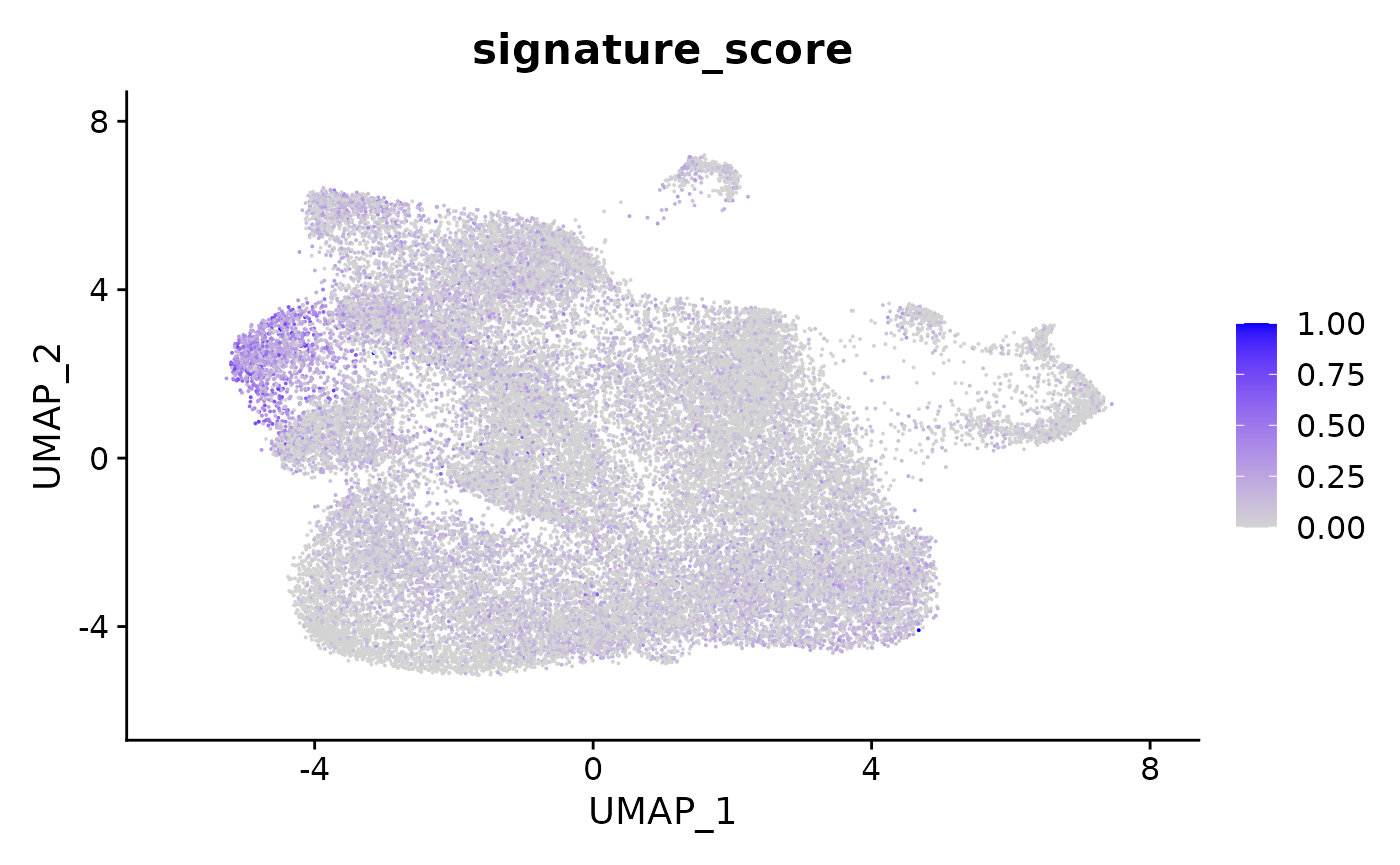

The cells could also be visualised using the popular and powerful ggplot package, enabling the researcher to use ggplot functions they were familiar with, and to customise the plot with great flexibility.

seurat_obj |>
  
  
  join_features(
    features = c("CD3D", "TRDC", "TRGC1", "TRGC2", "CD8A", "CD8B"),
    shape = "wide",
    assay = "SCT"
    
  ) |>
  
  mutate(signature_score =
           scales::rescale(CD3D + TRDC + TRGC1+ TRGC2, to=c(0,1)) -
           scales::rescale(CD8A + CD8B, to=c(0,1))
  ) |>
  
  mutate(signature_score = case_when(signature_score>0 ~ signature_score)) |>
  ggplot(aes(UMAP_1, UMAP_2, color = signature_score)) +
  geom_point(shape="." ) +
  scale_color_continuous_sequential(palette = "Blues", na.value = "grey") + 
  theme_bw()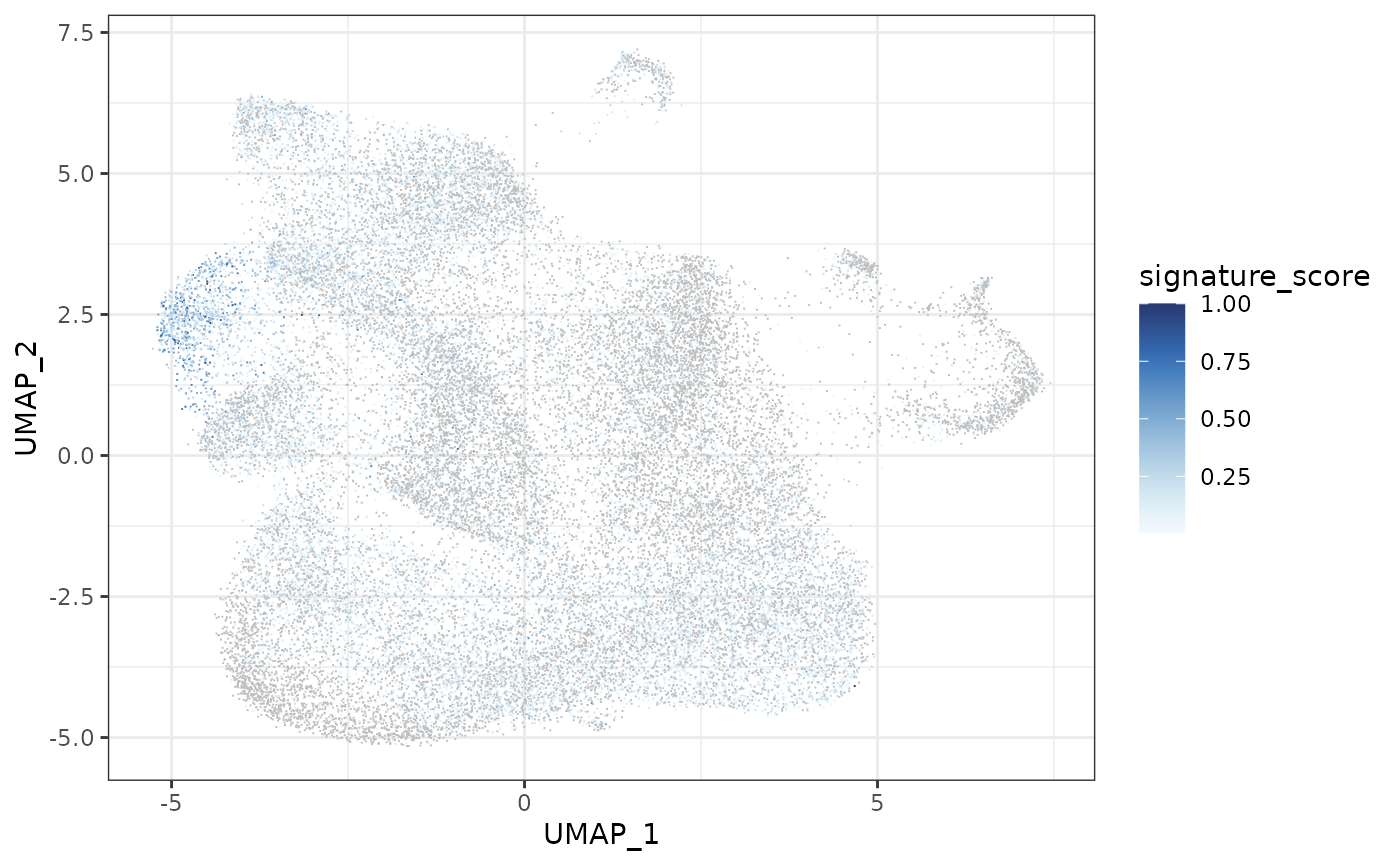

The gamma delta T cells (the blue cluster on the left with high signature score) could be interactively selected from the plot using the tidygate package.

seurat_obj |>
  
  
  join_features(
    features = c("CD3D", "TRDC", "TRGC1", "TRGC2", "CD8A", "CD8B"),
    shape = "wide",
    assay = "SCT"
    
  ) |>
  
  mutate(signature_score =
           scales::rescale(CD3D + TRDC + TRGC1+ TRGC2, to=c(0,1)) -
           scales::rescale(CD8A + CD8B, to=c(0,1))
  ) |>

  mutate(gate = tidygate::gate_int(
    UMAP_1, UMAP_2, 
    .size = 0.1, 
    .color =signature_score
  ))

Here we draw one gate but multiple gates can be drawn.

After the selection we can reload from file the gate drawn for reproducibility.

seurat_obj |>
  
  join_features(
    features = c("CD3D", "TRDC", "TRGC1", "TRGC2", "CD8A", "CD8B"),
    shape = "wide",
    assay = "SCT"
    
  ) |>
  
  mutate(signature_score =
           scales::rescale(CD3D + TRDC + TRGC1+ TRGC2, to=c(0,1)) -
           scales::rescale(CD8A + CD8B, to=c(0,1))
  ) |>

  mutate(gate = tidygate::gate_int(
    UMAP_1, UMAP_2, 
    .size = 0.1, 
    .color =signature_score,
    gate_list = iscb2022tidytranscriptomics::gate_seurat_obj
  ))

And the dataset could be filtered for just these cells using tidyverse filter.

seurat_obj |>
  
  
  join_features(
    features = c("CD3D", "TRDC", "TRGC1", "TRGC2", "CD8A", "CD8B"),
    shape = "wide",
    assay = "SCT"
    
  ) |>
  
  mutate(signature_score =
           scales::rescale(CD3D + TRDC + TRGC1+ TRGC2, to=c(0,1)) -
           scales::rescale(CD8A + CD8B, to=c(0,1))
  ) |>
  
  mutate(gate = tidygate::gate_int(UMAP_1, UMAP_2, gate_list = iscb2022tidytranscriptomics::gate_seurat_obj)) |> 
  
  filter(gate == 1)

## # A Seurat-tibble abstraction: 1,156 × 25
## # Features=6 | Active assay=SCT | Assays=RNA, SCT
##    .cell file  sample_id sample Barcode batch BCB    S.Score G2M.Score Phase
##    <chr> <chr> <chr>     <chr>  <chr>   <chr> <chr>    <dbl>     <dbl> <chr>
##  1 1_AA… ../d… SI-GA-H1… SI-GA… AAATGG… 1     BCB1… -0.0207    -0.0602 G1   
##  2 1_AC… ../d… SI-GA-H1… SI-GA… ACGATG… 1     BCB1…  0.0396    -0.0866 S    
##  3 1_AC… ../d… SI-GA-H1… SI-GA… ACGTAA… 1     BCB1… -0.00869   -0.140  G1   
##  4 1_AG… ../d… SI-GA-H1… SI-GA… AGCCAC… 1     BCB1… -0.00207   -0.0860 G1   
##  5 1_AG… ../d… SI-GA-H1… SI-GA… AGTAGT… 1     BCB1…  0.107     -0.0753 S    
##  6 1_AT… ../d… SI-GA-H1… SI-GA… ATCACG… 1     BCB1…  0.0103    -0.109  S    
##  7 1_AT… ../d… SI-GA-H1… SI-GA… ATTCGT… 1     BCB1… -0.0273    -0.0333 G1   
##  8 1_CA… ../d… SI-GA-H1… SI-GA… CATCCA… 1     BCB1…  0.0516    -0.131  S    
##  9 1_CC… ../d… SI-GA-H1… SI-GA… CCACAA… 1     BCB1…  0.0382    -0.0859 S    
## 10 1_CC… ../d… SI-GA-H1… SI-GA… CCGAAC… 1     BCB1…  0.0215    -0.0328 S    
## # … with 1,146 more rows, and 15 more variables: curated_cell_type <chr>,
## #   nCount_RNA <dbl>, nFeature_RNA <int>, nCount_SCT <dbl>, nFeature_SCT <int>,
## #   CD3D <dbl>, TRDC <dbl>, TRGC1 <dbl>, TRGC2 <dbl>, CD8A <dbl>, CD8B <dbl>,
## #   signature_score <dbl>, gate <int>, UMAP_1 <dbl>, UMAP_2 <dbl>

It was then possible to perform analyses on these gamma delta T cells by simply chaining further commands, such as below.

seurat_obj |>
  
  
  join_features(
    features = c("CD3D", "TRDC", "TRGC1", "TRGC2", "CD8A", "CD8B"),
    shape = "wide",
    assay = "SCT"
    
  ) |>
  
  mutate(signature_score =
           scales::rescale(CD3D + TRDC + TRGC1+ TRGC2, to=c(0,1)) -
           scales::rescale(CD8A + CD8B, to=c(0,1))
  ) |>
  
  mutate(gate = tidygate::gate_int(UMAP_1, UMAP_2, gate_list = iscb2022tidytranscriptomics::gate_seurat_obj) ) |> 
  
  filter(gate == 1) |>
  
  # Reanalyse
  NormalizeData(assay="RNA") |> 
  FindVariableFeatures(nfeatures = 100, assay="RNA") |>
  SplitObject(split.by = "file") |> 
  RunFastMNN(assay="RNA") |> 
  RunUMAP(reduction = "mnn", dims = 1:20) |> 
  FindNeighbors(dims = 1:20, reduction = "mnn") |> 
  FindClusters(resolution = 0.3)

For comparison, we show the alternative using base R and Seurat

counts_positive <- 
  GetAssayData(seurat_obj, assay="SCT")[c("CD3D", "TRDC", "TRGC1", "TRGC2"),] |> 
  colSums() |> 
  scales::rescale(to=c(0,1)) 

counts_negative <- 
  GetAssayData(seurat_obj, assay="SCT")[c("CD8A", "CD8B"),] |> 
  colSums()  |> 
  scales::rescale(to=c(0,1)) 

seurat_obj$signature_score <- counts_positive - counts_negative

p <- FeaturePlot(seurat_obj, features = "signature_score")

# This is not reproducible (in contrast to tidygate)
seurat_obj$within_gate <- colnames(seurat_obj) %in% CellSelector(plot = p)

seurat_obj |> 
  subset(within_gate == TRUE) |>
  
  # Reanalyse
  NormalizeData(assay="RNA") |> 
  FindVariableFeatures(nfeatures = 100, assay="RNA") |>
  SplitObject(split.by = "file") |> 
  RunFastMNN(assay="RNA") |> 
  RunUMAP(reduction = "mnn", dims = 1:20) |> 
  FindNeighbors(dims = 1:20, reduction = "mnn") |> 
  FindClusters(resolution = 0.3)

As a final note, it’s also possible to do complex and powerful things in a simple way, due to the integration of the tidy transcriptomics packages with the tidy universe. As one example, we can visualise the cells as a 3D plot using plotly.

The example data we’ve been using only contains a few genes, for the sake of time and size in this demonstration, but below is how you could generate the 3 dimensions needed for 3D plot with a full dataset.

single_cell_object |> 
  RunUMAP(dims = 1:30, n.components = 3L, spread = 0.5,min.dist  = 0.01, n.neighbors = 10L)

We’ll demonstrate creating a 3D plot using some data that has 3 UMAP dimensions.

pbmc <- iscb2022tidytranscriptomics::seurat_obj_UMAP3

pbmc |>
    
  plot_ly(
    x = ~`UMAP_1`,
    y = ~`UMAP_2`,
    z = ~`UMAP_3`,
    color = ~curated_cell_type,
    colors = dittoSeq::dittoColors()
  ) |> 
  
   add_markers(size = I(1))

Exercises

What proportion of all cells are gamma-delta T cells?
There is a cluster of cells characterised by a low RNA output (nCount_RNA). Use tidygate to identify the cell composition (curated_cell_type) of that cluster.

Session Information

sessionInfo()

## R version 4.1.2 (2021-11-01)
## Platform: x86_64-pc-linux-gnu (64-bit)
## Running under: Ubuntu 20.04.3 LTS
## 
## Matrix products: default
## BLAS/LAPACK: /usr/lib/x86_64-linux-gnu/openblas-pthread/libopenblasp-r0.3.8.so
## 
## locale:
##  [1] LC_CTYPE=en_US.UTF-8       LC_NUMERIC=C              
##  [3] LC_TIME=en_US.UTF-8        LC_COLLATE=en_US.UTF-8    
##  [5] LC_MONETARY=en_US.UTF-8    LC_MESSAGES=en_US.UTF-8   
##  [7] LC_PAPER=en_US.UTF-8       LC_NAME=C                 
##  [9] LC_ADDRESS=C               LC_TELEPHONE=C            
## [11] LC_MEASUREMENT=en_US.UTF-8 LC_IDENTIFICATION=C       
## 
## attached base packages:
## [1] stats     graphics  grDevices utils     datasets  methods   base     
## 
## other attached packages:
##  [1] tidyseurat_0.5.1     ttservice_0.1.2      dittoSeq_1.6.0      
##  [4] SeuratWrappers_0.3.0 colorspace_2.0-3     dplyr_1.0.8         
##  [7] plotly_4.10.0        ggplot2_3.3.5        SeuratObject_4.0.4  
## [10] Seurat_4.1.0        
## 
## loaded via a namespace (and not attached):
##   [1] systemfonts_1.0.4                  plyr_1.8.6                        
##   [3] igraph_1.2.11                      lazyeval_0.2.2                    
##   [5] splines_4.1.2                      crosstalk_1.2.0                   
##   [7] iscb2022tidytranscriptomics_0.12.3 listenv_0.8.0                     
##   [9] scattermore_0.8                    GenomeInfoDb_1.30.1               
##  [11] digest_0.6.29                      htmltools_0.5.2                   
##  [13] viridis_0.6.2                      fansi_1.0.2                       
##  [15] magrittr_2.0.2                     memoise_2.0.1                     
##  [17] tensor_1.5                         cluster_2.1.2                     
##  [19] ROCR_1.0-11                        remotes_2.4.2                     
##  [21] globals_0.14.0                     matrixStats_0.61.0                
##  [23] R.utils_2.11.0                     pkgdown_2.0.2                     
##  [25] spatstat.sparse_2.1-0              ggrepel_0.9.1                     
##  [27] textshaping_0.3.6                  xfun_0.29                         
##  [29] RCurl_1.98-1.6                     crayon_1.5.0                      
##  [31] jsonlite_1.7.3                     spatstat.data_2.1-2               
##  [33] survival_3.2-13                    zoo_1.8-9                         
##  [35] glue_1.6.1                         polyclip_1.10-0                   
##  [37] gtable_0.3.0                       zlibbioc_1.40.0                   
##  [39] XVector_0.34.0                     leiden_0.3.9                      
##  [41] DelayedArray_0.20.0                future.apply_1.8.1                
##  [43] SingleCellExperiment_1.16.0        BiocGenerics_0.40.0               
##  [45] abind_1.4-5                        scales_1.1.1                      
##  [47] pheatmap_1.0.12                    spatstat.random_2.1-0             
##  [49] miniUI_0.1.1.1                     Rcpp_1.0.8                        
##  [51] viridisLite_0.4.0                  xtable_1.8-4                      
##  [53] reticulate_1.24                    spatstat.core_2.4-0               
##  [55] rsvd_1.0.5                         stats4_4.1.2                      
##  [57] htmlwidgets_1.5.4                  httr_1.4.2                        
##  [59] RColorBrewer_1.1-2                 ellipsis_0.3.2                    
##  [61] ica_1.0-2                          farver_2.1.0                      
##  [63] pkgconfig_2.0.3                    R.methodsS3_1.8.1                 
##  [65] sass_0.4.0                         uwot_0.1.11                       
##  [67] deldir_1.0-6                       utf8_1.2.2                        
##  [69] labeling_0.4.2                     tidyselect_1.1.1                  
##  [71] rlang_1.0.1                        reshape2_1.4.4                    
##  [73] later_1.3.0                        munsell_0.5.0                     
##  [75] tools_4.1.2                        cachem_1.0.6                      
##  [77] cli_3.2.0                          generics_0.1.2                    
##  [79] ggridges_0.5.3                     evaluate_0.15                     
##  [81] stringr_1.4.0                      fastmap_1.1.0                     
##  [83] yaml_2.3.5                         ragg_1.2.2                        
##  [85] goftest_1.2-3                      knitr_1.37                        
##  [87] fs_1.5.2                           fitdistrplus_1.1-6                
##  [89] purrr_0.3.4                        RANN_2.6.1                        
##  [91] pbapply_1.5-0                      future_1.24.0                     
##  [93] nlme_3.1-155                       mime_0.12                         
##  [95] R.oo_1.24.0                        compiler_4.1.2                    
##  [97] png_0.1-7                          spatstat.utils_2.3-0              
##  [99] tibble_3.1.6                       bslib_0.3.1                       
## [101] stringi_1.7.6                      highr_0.9                         
## [103] desc_1.4.0                         tidygate_0.4.9                    
## [105] lattice_0.20-45                    Matrix_1.4-0                      
## [107] vctrs_0.3.8                        pillar_1.7.0                      
## [109] lifecycle_1.0.1                    BiocManager_1.30.16               
## [111] spatstat.geom_2.3-2                lmtest_0.9-39                     
## [113] jquerylib_0.1.4                    RcppAnnoy_0.0.19                  
## [115] bitops_1.0-7                       data.table_1.14.2                 
## [117] cowplot_1.1.1                      irlba_2.3.5                       
## [119] GenomicRanges_1.46.1               httpuv_1.6.5                      
## [121] patchwork_1.1.1                    R6_2.5.1                          
## [123] promises_1.2.0.1                   KernSmooth_2.23-20                
## [125] gridExtra_2.3                      IRanges_2.28.0                    
## [127] parallelly_1.30.0                  codetools_0.2-18                  
## [129] MASS_7.3-55                        SummarizedExperiment_1.24.0       
## [131] rprojroot_2.0.2                    withr_2.4.3                       
## [133] sctransform_0.3.3                  GenomeInfoDbData_1.2.7            
## [135] S4Vectors_0.32.3                   mgcv_1.8-38                       
## [137] parallel_4.1.2                     grid_4.1.2                        
## [139] rpart_4.1.16                       tidyr_1.2.0                       
## [141] rmarkdown_2.11                     MatrixGenerics_1.6.0              
## [143] Rtsne_0.15                         Biobase_2.54.0                    
## [145] shiny_1.7.1

References

Butler, Andrew, Paul Hoffman, Peter Smibert, Efthymia Papalexi, and Rahul Satija. 2018. “Integrating Single-Cell Transcriptomic Data Across Different Conditions, Technologies, and Species.” Nature Biotechnology 36 (5): 411–20.

Pizzolato, Gabriele, Hannah Kaminski, Marie Tosolini, Don-Marc Franchini, Fréderic Pont, Fréderic Martins, Carine Valle, et al. 2019. “Single-Cell RNA Sequencing Unveils the Shared and the Distinct Cytotoxic Hallmarks of Human TCRV\(\updelta\)1 and TCRV\(\updelta\)2 \(\upgamma\)\(\updelta\) t Lymphocytes.” Proceedings of the National Academy of Sciences, May, 201818488. https://doi.org/10.1073/pnas.1818488116.

Stuart, Tim, Andrew Butler, Paul Hoffman, Christoph Hafemeister, Efthymia Papalexi, William M Mauck III, Yuhan Hao, Marlon Stoeckius, Peter Smibert, and Rahul Satija. 2019. “Comprehensive Integration of Single-Cell Data.” Cell 177 (7): 1888–1902.

Wickham, Hadley, Mara Averick, Jennifer Bryan, Winston Chang, Lucy D’Agostino McGowan, Romain François, Garrett Grolemund, et al. 2019. “Welcome to the Tidyverse.” Journal of Open Source Software 4 (43): 1686.

<maria.doyle at petermac.org>↩︎
<mangiola.s at wehi.edu.au>↩︎

Maria Doyle, Peter MacCallum Cancer Centre¹

Stefano Mangiola, Walter and Eliza Hall Institute²

Instructors

Workshop goals and objectives

What you will learn

What you will not learn

Slides

Getting started

Cloud

Local

Introduction to tidyseurat

Tidyverse commands

Case study

Data pre-processing

Analyse custom signature

Exercises

Tidy Transcriptomics for Single-cell RNA Sequencing Analyses

Maria Doyle, Peter MacCallum Cancer Centre1

Stefano Mangiola, Walter and Eliza Hall Institute2

Instructors

Workshop goals and objectives

What you will learn

What you will not learn

Slides

Getting started

Cloud

Local

Introduction to tidyseurat

Tidyverse commands

Case study

Data pre-processing

Analyse custom signature

Exercises

Maria Doyle, Peter MacCallum Cancer Centre¹

Stefano Mangiola, Walter and Eliza Hall Institute²