Tidy Transcriptomics For Single-Cell RNA Sequencing Analyses

Workshop introduction

BioC2022 tidybulk

Instructors

Dr. Stefano Mangiola is currently a Postdoctoral researcher in the laboratory of Prof. Tony Papenfuss at the Walter and Eliza Hall Institute in Melbourne, Australia. His background spans from biotechnology to bioinformatics and biostatistics. His research focuses on prostate and breast tumour microenvironment, the development of statistical models for the analysis of RNA sequencing data, and data analysis and visualisation interfaces.

Dr. Maria Doyle is the Application and Training Specialist for Research Computing at the Peter MacCallum Cancer Centre in Melbourne, Australia. She has a PhD in Molecular Biology and currently works in bioinformatics and data science education and training. She is passionate about supporting researchers, reproducible research, open source and tidy data.

Description

This tutorial will showcase analysis of single-cell RNA sequencing data following the tidy data paradigm. The tidy data paradigm provides a standard way to organise data values within a dataset, where each variable is a column, each observation is a row, and data is manipulated using an easy-to-understand vocabulary. Most importantly, the data structure remains consistent across manipulation and analysis functions.

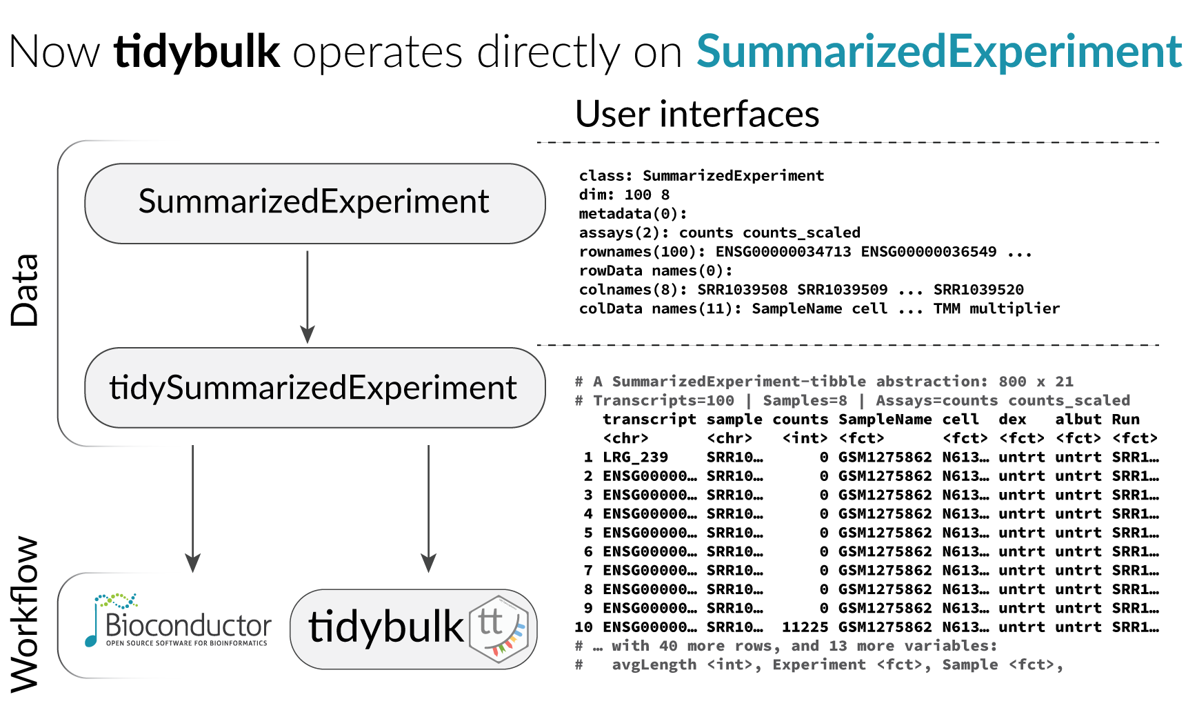
This can be achieved with the integration of packages present in the R CRAN and Bioconductor ecosystem, including tidySingleCellExperiment, tidySummarizedExperiment, tidybulk and tidyverse. These packages are part of the tidytranscriptomics suite that introduces a tidy approach to RNA sequencing data representation and analysis. For more information see the tidy transcriptomics blog.

Pre-requisites

Basic familiarity with single-cell transcriptomic analyses
Basic familiarity with tidyverse

Goals and objectives

To approach single-cell data representation and analysis through a tidy data paradigm, integrating tidyverse with tidySingleCellExperiment.
Compare SingleCellExperiment and tidy representation
Apply tidy functions to SingleCellExperiment objects
Reproduce a real-world case study that showcases the power of tidy single-cell methods

What you will learn

Basic tidy operations possible with tidySingleCellExperiment
The differences between SingleCellExperiment representation and tidy representation
How to interface SingleCellExperiment with tidy manipulation and visualisation
A real-world case study that will showcase the power of tidy single-cell methods compared with base/ad-hoc methods

What you will not learn

The molecular technology of single-cell sequencing
The fundamentals of single-cell data analysis
The fundamentals of tidy data analysis

This workshop will demonstrate a real-world example of using tidy transcriptomics packages to analyse single cell data. This workshop is not a step-by-step introduction in how to perform single-cell analysis. For an overview of single-cell analysis steps performed in a tidy way please see the ISMB2021 workshop.

Getting started

Cloud

Easiest way to run this material. We will use the Orchestra Cloud platform during the BioC2022 workshop.

Go to Orchestra.
Log in.
Find the workshop. In the search box type bioc2022, sort by Created column, and select the most recently created workshop called “BioC2022: Tidy Transcriptomics For Single-Cell RNA Sequencing Analyses” There are several tidy transcriptomics workshops. Be sure to select the BioC2022 one with the most recent created date.
Click “Launch” (may take a minute or two).
Follow instructions.. Do not share your personalized URL for the RStudio session, or use the trainers, as only one browser at a time can be connected.
Open tidytranscriptomics_case_study.Rmd in bioc2022_tidytranscriptomcs/vignettes folder

Local

We will use the Orchestra Cloud platform during the BioC2022 workshop and this method is available if you want to run the material after the workshop. If you want to install on your own computer, see instructions here.

Alternatively, you can view the material at the workshop webpage here.

Slides

The embedded slides below may take a minute to appear. You can also view or download here.

Part 1 Introduction to tidySingleCellExperiment

# Load packages
library(SingleCellExperiment)
library(ggplot2)
library(plotly)
library(dplyr)
library(colorspace)
library(dittoSeq)

SingleCellExperiment is a very popular analysis toolkit for single cell RNA sequencing data (Butler et al. 2018; Stuart et al. 2019).

Here we load single-cell data in SingleCellExperiment object format. This data is peripheral blood mononuclear cells (PBMCs) from metastatic breast cancer patients.

# load single cell RNA sequencing data
sce_obj <- bioc2022tidytranscriptomics::sce_obj

# take a look
sce_obj

## class: SingleCellExperiment 
## dim: 482 3580 
## metadata(0):
## assays(2): counts logcounts
## rownames(482): HBB HBA2 ... TRGC2 CD8A
## rowData names(0):
## colnames(3580): 1_AAATGGACAAGTTCGT-1 1_AACAAGAGTGTTGAGG-1 ...
##   10_TTTGTTGGTACACGTT-1 10_TTTGTTGGTGATAGAT-1
## colData names(15): Barcode batch ... treatment sample
## reducedDimNames(1): UMAP
## mainExpName: SCT
## altExpNames(1): RNA

tidySingleCellExperiment provides a bridge between the SingleCellExperiment single-cell package and the tidyverse (Wickham et al. 2019). It creates an invisible layer that enables viewing the SingleCellExperiment object as a tidyverse tibble, and provides SingleCellExperiment-compatible dplyr, tidyr, ggplot and plotly functions.

If we load the tidySingleCellExperiment package and then view the single cell data, it now displays as a tibble.

library(tidySingleCellExperiment)

sce_obj

## # A SingleCellExperiment-tibble abstraction: 3,580 × 18
## # Features=482 | Cells=3580 | Assays=counts, logcounts
##    .cell      Barcode batch BCB    S.Score G2M.S…¹ Phase cell_…² nCoun…³ nFeat…⁴
##    <chr>      <fct>   <fct> <fct>    <dbl>   <dbl> <fct> <fct>     <int>   <int>
##  1 1_AAATGGA… AAATGG… 1     BCB1… -2.07e-2 -0.0602 G1    TCR_V_…     215      36
##  2 1_AACAAGA… AACAAG… 1     BCB1…  2.09e-2 -0.0357 S     CD8+_t…     145      41
##  3 1_AACGTCA… AACGTC… 1     BCB1… -2.54e-2 -0.133  G1    CD8+_h…     356      44
##  4 1_AACTTCT… AACTTC… 1     BCB1…  2.85e-2 -0.163  S     CD8+_t…     385      58
##  5 1_AAGTCGT… AAGTCG… 1     BCB1… -2.30e-2 -0.0581 G1    MAIT        352      42
##  6 1_AATGAAG… AATGAA… 1     BCB1…  1.09e-2 -0.0621 S     CD4+_r…     335      40
##  7 1_ACAAAGA… ACAAAG… 1     BCB1… -2.06e-2 -0.0409 G1    CD4+_T…     242      39
##  8 1_ACACGCG… ACACGC… 1     BCB1… -3.95e-4 -0.176  G1    CD8+_h…     438      45
##  9 1_ACATGCA… ACATGC… 1     BCB1… -4.09e-2 -0.0829 G1    CD4+_r…     180      39
## 10 1_ACGATCA… ACGATC… 1     BCB1…  8.82e-2 -0.0397 S     CD4+_r…      82      34
## # … with 3,570 more rows, 8 more variables: nCount_SCT <int>,
## #   nFeature_SCT <int>, ident <fct>, file <chr>, treatment <chr>,
## #   sample <glue>, UMAP_1 <dbl>, UMAP_2 <dbl>, and abbreviated variable names
## #   ¹G2M.Score, ²cell_type, ³nCount_RNA, ⁴nFeature_RNA
## # ℹ Use `print(n = ...)` to see more rows, and `colnames()` to see all variable names

If we want to revert to the standard SingleCellExperiment view we can do that.

options("restore_SingleCellExperiment_show" = TRUE)
sce_obj

## class: SingleCellExperiment 
## dim: 482 3580 
## metadata(0):
## assays(2): counts logcounts
## rownames(482): HBB HBA2 ... TRGC2 CD8A
## rowData names(0):
## colnames(3580): 1_AAATGGACAAGTTCGT-1 1_AACAAGAGTGTTGAGG-1 ...
##   10_TTTGTTGGTACACGTT-1 10_TTTGTTGGTGATAGAT-1
## colData names(15): Barcode batch ... treatment sample

If we want to revert back to tidy SingleCellExperiment view we can.

options("restore_SingleCellExperiment_show" = FALSE)
sce_obj

## # A SingleCellExperiment-tibble abstraction: 3,580 × 18
## # Features=482 | Cells=3580 | Assays=counts, logcounts
##    .cell      Barcode batch BCB    S.Score G2M.S…¹ Phase cell_…² nCoun…³ nFeat…⁴
##    <chr>      <fct>   <fct> <fct>    <dbl>   <dbl> <fct> <fct>     <int>   <int>
##  1 1_AAATGGA… AAATGG… 1     BCB1… -2.07e-2 -0.0602 G1    TCR_V_…     215      36
##  2 1_AACAAGA… AACAAG… 1     BCB1…  2.09e-2 -0.0357 S     CD8+_t…     145      41
##  3 1_AACGTCA… AACGTC… 1     BCB1… -2.54e-2 -0.133  G1    CD8+_h…     356      44
##  4 1_AACTTCT… AACTTC… 1     BCB1…  2.85e-2 -0.163  S     CD8+_t…     385      58
##  5 1_AAGTCGT… AAGTCG… 1     BCB1… -2.30e-2 -0.0581 G1    MAIT        352      42
##  6 1_AATGAAG… AATGAA… 1     BCB1…  1.09e-2 -0.0621 S     CD4+_r…     335      40
##  7 1_ACAAAGA… ACAAAG… 1     BCB1… -2.06e-2 -0.0409 G1    CD4+_T…     242      39
##  8 1_ACACGCG… ACACGC… 1     BCB1… -3.95e-4 -0.176  G1    CD8+_h…     438      45
##  9 1_ACATGCA… ACATGC… 1     BCB1… -4.09e-2 -0.0829 G1    CD4+_r…     180      39
## 10 1_ACGATCA… ACGATC… 1     BCB1…  8.82e-2 -0.0397 S     CD4+_r…      82      34
## # … with 3,570 more rows, 8 more variables: nCount_SCT <int>,
## #   nFeature_SCT <int>, ident <fct>, file <chr>, treatment <chr>,
## #   sample <glue>, UMAP_1 <dbl>, UMAP_2 <dbl>, and abbreviated variable names
## #   ¹G2M.Score, ²cell_type, ³nCount_RNA, ⁴nFeature_RNA
## # ℹ Use `print(n = ...)` to see more rows, and `colnames()` to see all variable names

It can be interacted with using SingleCellExperiment commands such as assays.

assays(sce_obj)

## List of length 2
## names(2): counts logcounts

We can also interact with our object as we do with any tidyverse tibble.

Tidyverse commands

We can use tidyverse commands, such as filter, select and mutate to explore the tidySingleCellExperiment object. Some examples are shown below and more can be seen at the tidySingleCellExperiment website here.

We can use filter to choose rows, for example, to see just the rows for the cells in G1 cell-cycle stage.

sce_obj |> filter(Phase == "G1")

## # A SingleCellExperiment-tibble abstraction: 1,859 × 18
## # Features=482 | Cells=1859 | Assays=counts, logcounts
##    .cell      Barcode batch BCB    S.Score G2M.S…¹ Phase cell_…² nCoun…³ nFeat…⁴
##    <chr>      <fct>   <fct> <fct>    <dbl>   <dbl> <fct> <fct>     <int>   <int>
##  1 1_AAATGGA… AAATGG… 1     BCB1… -2.07e-2 -0.0602 G1    TCR_V_…     215      36
##  2 1_AACGTCA… AACGTC… 1     BCB1… -2.54e-2 -0.133  G1    CD8+_h…     356      44
##  3 1_AAGTCGT… AAGTCG… 1     BCB1… -2.30e-2 -0.0581 G1    MAIT        352      42
##  4 1_ACAAAGA… ACAAAG… 1     BCB1… -2.06e-2 -0.0409 G1    CD4+_T…     242      39
##  5 1_ACACGCG… ACACGC… 1     BCB1… -3.95e-4 -0.176  G1    CD8+_h…     438      45
##  6 1_ACATGCA… ACATGC… 1     BCB1… -4.09e-2 -0.0829 G1    CD4+_r…     180      39
##  7 1_ACGTAAC… ACGTAA… 1     BCB1… -8.69e-3 -0.140  G1    TCR_V_…     187      57
##  8 1_AGAGAAT… AGAGAA… 1     BCB1… -5.14e-3 -0.102  G1    CD8+_t…     155      40
##  9 1_AGATCCA… AGATCC… 1     BCB1… -1.17e-2 -0.155  G1    CD8+_h…     433      42
## 10 1_AGCCAAT… AGCCAA… 1     BCB1… -3.61e-2 -0.207  G1    CD4+_T…     353      43
## # … with 1,849 more rows, 8 more variables: nCount_SCT <int>,
## #   nFeature_SCT <int>, ident <fct>, file <chr>, treatment <chr>,
## #   sample <glue>, UMAP_1 <dbl>, UMAP_2 <dbl>, and abbreviated variable names
## #   ¹G2M.Score, ²cell_type, ³nCount_RNA, ⁴nFeature_RNA
## # ℹ Use `print(n = ...)` to see more rows, and `colnames()` to see all variable names

We can use select to view columns, for example, to see the filename, total cellular RNA abundance and cell phase.

If we use select we will also get any view-only columns returned, such as the UMAP columns generated during the preprocessing.

sce_obj |> select(.cell, file, nCount_RNA, Phase)

## # A SingleCellExperiment-tibble abstraction: 3,580 × 6
## # Features=482 | Cells=3580 | Assays=counts, logcounts
##    .cell                file                         nCoun…¹ Phase UMAP_1 UMAP_2
##    <chr>                <chr>                          <int> <fct>  <dbl>  <dbl>
##  1 1_AAATGGACAAGTTCGT-1 ../data/single_cell/SI-GA-H…     215 G1    -3.73  -1.59 
##  2 1_AACAAGAGTGTTGAGG-1 ../data/single_cell/SI-GA-H…     145 S      0.798 -0.151
##  3 1_AACGTCAGTCTATGAC-1 ../data/single_cell/SI-GA-H…     356 G1    -0.292  0.515
##  4 1_AACTTCTCACGCTGAC-1 ../data/single_cell/SI-GA-H…     385 S      0.372  2.34 
##  5 1_AAGTCGTGTGTTGCCG-1 ../data/single_cell/SI-GA-H…     352 G1    -1.63  -0.236
##  6 1_AATGAAGCATCCAACA-1 ../data/single_cell/SI-GA-H…     335 S      0.822  2.90 
##  7 1_ACAAAGAGTCGTACTA-1 ../data/single_cell/SI-GA-H…     242 G1     3.28   3.97 
##  8 1_ACACGCGCAGGTACGA-1 ../data/single_cell/SI-GA-H…     438 G1    -3.65  -0.192
##  9 1_ACATGCATCACTTTGT-1 ../data/single_cell/SI-GA-H…     180 G1    -0.273  4.09 
## 10 1_ACGATCATCGACGAGA-1 ../data/single_cell/SI-GA-H…      82 S     -0.816  2.90 
## # … with 3,570 more rows, and abbreviated variable name ¹nCount_RNA
## # ℹ Use `print(n = ...)` to see more rows

We can use mutate to create a column. For example, we could create a new Phase_l column that contains a lower-case version of Phase.

sce_obj |>
  mutate(Phase_l = tolower(Phase)) |>
  select(.cell, Phase, Phase_l)

## # A SingleCellExperiment-tibble abstraction: 3,580 × 5
## # Features=482 | Cells=3580 | Assays=counts, logcounts
##    .cell                Phase Phase_l UMAP_1 UMAP_2
##    <chr>                <fct> <chr>    <dbl>  <dbl>
##  1 1_AAATGGACAAGTTCGT-1 G1    g1      -3.73  -1.59 
##  2 1_AACAAGAGTGTTGAGG-1 S     s        0.798 -0.151
##  3 1_AACGTCAGTCTATGAC-1 G1    g1      -0.292  0.515
##  4 1_AACTTCTCACGCTGAC-1 S     s        0.372  2.34 
##  5 1_AAGTCGTGTGTTGCCG-1 G1    g1      -1.63  -0.236
##  6 1_AATGAAGCATCCAACA-1 S     s        0.822  2.90 
##  7 1_ACAAAGAGTCGTACTA-1 G1    g1       3.28   3.97 
##  8 1_ACACGCGCAGGTACGA-1 G1    g1      -3.65  -0.192
##  9 1_ACATGCATCACTTTGT-1 G1    g1      -0.273  4.09 
## 10 1_ACGATCATCGACGAGA-1 S     s       -0.816  2.90 
## # … with 3,570 more rows
## # ℹ Use `print(n = ...)` to see more rows

We can use tidyverse commands to polish an annotation column. We will extract the sample, and group information from the file name column into separate columns.

# First take a look at the file column
sce_obj |> select(.cell, file)

## # A SingleCellExperiment-tibble abstraction: 3,580 × 4
## # Features=482 | Cells=3580 | Assays=counts, logcounts
##    .cell                file                                       UMAP_1 UMAP_2
##    <chr>                <chr>                                       <dbl>  <dbl>
##  1 1_AAATGGACAAGTTCGT-1 ../data/single_cell/SI-GA-H1/outs/raw_fea… -3.73  -1.59 
##  2 1_AACAAGAGTGTTGAGG-1 ../data/single_cell/SI-GA-H1/outs/raw_fea…  0.798 -0.151
##  3 1_AACGTCAGTCTATGAC-1 ../data/single_cell/SI-GA-H1/outs/raw_fea… -0.292  0.515
##  4 1_AACTTCTCACGCTGAC-1 ../data/single_cell/SI-GA-H1/outs/raw_fea…  0.372  2.34 
##  5 1_AAGTCGTGTGTTGCCG-1 ../data/single_cell/SI-GA-H1/outs/raw_fea… -1.63  -0.236
##  6 1_AATGAAGCATCCAACA-1 ../data/single_cell/SI-GA-H1/outs/raw_fea…  0.822  2.90 
##  7 1_ACAAAGAGTCGTACTA-1 ../data/single_cell/SI-GA-H1/outs/raw_fea…  3.28   3.97 
##  8 1_ACACGCGCAGGTACGA-1 ../data/single_cell/SI-GA-H1/outs/raw_fea… -3.65  -0.192
##  9 1_ACATGCATCACTTTGT-1 ../data/single_cell/SI-GA-H1/outs/raw_fea… -0.273  4.09 
## 10 1_ACGATCATCGACGAGA-1 ../data/single_cell/SI-GA-H1/outs/raw_fea… -0.816  2.90 
## # … with 3,570 more rows
## # ℹ Use `print(n = ...)` to see more rows

# Create column for sample
sce_obj <- sce_obj |>
  # Extract sample
  extract(file, "sample", "../data/.*/([a-zA-Z0-9_-]+)/outs.+", remove = FALSE)

# Take a look
sce_obj |> select(.cell, sample, everything())

## # A SingleCellExperiment-tibble abstraction: 3,580 × 18
## # Features=482 | Cells=3580 | Assays=counts, logcounts
##    .cell       sample Barcode batch BCB    S.Score G2M.S…¹ Phase cell_…² nCoun…³
##    <chr>       <chr>  <fct>   <fct> <fct>    <dbl>   <dbl> <fct> <fct>     <int>
##  1 1_AAATGGAC… SI-GA… AAATGG… 1     BCB1… -2.07e-2 -0.0602 G1    TCR_V_…     215
##  2 1_AACAAGAG… SI-GA… AACAAG… 1     BCB1…  2.09e-2 -0.0357 S     CD8+_t…     145
##  3 1_AACGTCAG… SI-GA… AACGTC… 1     BCB1… -2.54e-2 -0.133  G1    CD8+_h…     356
##  4 1_AACTTCTC… SI-GA… AACTTC… 1     BCB1…  2.85e-2 -0.163  S     CD8+_t…     385
##  5 1_AAGTCGTG… SI-GA… AAGTCG… 1     BCB1… -2.30e-2 -0.0581 G1    MAIT        352
##  6 1_AATGAAGC… SI-GA… AATGAA… 1     BCB1…  1.09e-2 -0.0621 S     CD4+_r…     335
##  7 1_ACAAAGAG… SI-GA… ACAAAG… 1     BCB1… -2.06e-2 -0.0409 G1    CD4+_T…     242
##  8 1_ACACGCGC… SI-GA… ACACGC… 1     BCB1… -3.95e-4 -0.176  G1    CD8+_h…     438
##  9 1_ACATGCAT… SI-GA… ACATGC… 1     BCB1… -4.09e-2 -0.0829 G1    CD4+_r…     180
## 10 1_ACGATCAT… SI-GA… ACGATC… 1     BCB1…  8.82e-2 -0.0397 S     CD4+_r…      82
## # … with 3,570 more rows, 8 more variables: nFeature_RNA <int>,
## #   nCount_SCT <int>, nFeature_SCT <int>, ident <fct>, file <chr>,
## #   treatment <chr>, UMAP_1 <dbl>, UMAP_2 <dbl>, and abbreviated variable names
## #   ¹G2M.Score, ²cell_type, ³nCount_RNA
## # ℹ Use `print(n = ...)` to see more rows, and `colnames()` to see all variable names

We could use tidyverse unite to combine columns, for example to create a new column for sample id combining the sample and patient id (BCB) columns.

sce_obj <- sce_obj |> unite("sample_id", sample, BCB, remove = FALSE)

# Take a look
sce_obj |> select(.cell, sample_id, sample, BCB)

## # A SingleCellExperiment-tibble abstraction: 3,580 × 6
## # Features=482 | Cells=3580 | Assays=counts, logcounts
##    .cell                sample_id       sample   BCB    UMAP_1 UMAP_2
##    <chr>                <chr>           <chr>    <fct>   <dbl>  <dbl>
##  1 1_AAATGGACAAGTTCGT-1 SI-GA-H1_BCB102 SI-GA-H1 BCB102 -3.73  -1.59 
##  2 1_AACAAGAGTGTTGAGG-1 SI-GA-H1_BCB102 SI-GA-H1 BCB102  0.798 -0.151
##  3 1_AACGTCAGTCTATGAC-1 SI-GA-H1_BCB102 SI-GA-H1 BCB102 -0.292  0.515
##  4 1_AACTTCTCACGCTGAC-1 SI-GA-H1_BCB102 SI-GA-H1 BCB102  0.372  2.34 
##  5 1_AAGTCGTGTGTTGCCG-1 SI-GA-H1_BCB102 SI-GA-H1 BCB102 -1.63  -0.236
##  6 1_AATGAAGCATCCAACA-1 SI-GA-H1_BCB102 SI-GA-H1 BCB102  0.822  2.90 
##  7 1_ACAAAGAGTCGTACTA-1 SI-GA-H1_BCB102 SI-GA-H1 BCB102  3.28   3.97 
##  8 1_ACACGCGCAGGTACGA-1 SI-GA-H1_BCB102 SI-GA-H1 BCB102 -3.65  -0.192
##  9 1_ACATGCATCACTTTGT-1 SI-GA-H1_BCB102 SI-GA-H1 BCB102 -0.273  4.09 
## 10 1_ACGATCATCGACGAGA-1 SI-GA-H1_BCB102 SI-GA-H1 BCB102 -0.816  2.90 
## # … with 3,570 more rows
## # ℹ Use `print(n = ...)` to see more rows

Part 2 Signature visualisation

Data pre-processing

The object sce_obj we’ve been using was created as part of a study on breast cancer systemic immune response. Peripheral blood mononuclear cells have been sequenced for RNA at the single-cell level. The steps used to generate the object are summarised below.

scran, scater, and DropletsUtils packages have been used to eliminate empty droplets and dead cells. Samples were individually quality checked and cells were filtered for good gene coverage.
Variable features were identified using modelGeneVar.
Read counts were scaled and normalised using logNormCounts from scuttle.
Data integration was performed using fastMNN with default parameters.
PCA performed to reduce feature dimensionality.
Nearest-neighbor cell networks were calculated using 30 principal components.
2 UMAP dimensions were calculated using 30 principal components.
Cells with similar transcriptome profiles were grouped into clusters using Louvain clustering from scran.

Analyse custom signature

The researcher analysing this dataset wanted to identify gamma delta T cells using a gene signature from a published paper (Pizzolato et al. 2019). We’ll show how that can be done here.

With tidySingleCellExperiment’s join_features we can view the counts for genes in the signature as columns joined to our single cell tibble.

sce_obj |>
  join_features(c("CD3D", "TRDC", "TRGC1", "TRGC2", "CD8A", "CD8B"), shape = "wide")

## # A SingleCellExperiment-tibble abstraction: 3,580 × 25
## # Features=482 | Cells=3580 | Assays=counts, logcounts
##    .cell      Barcode batch sampl…¹ BCB    S.Score G2M.S…² Phase cell_…³ nCoun…⁴
##    <chr>      <fct>   <fct> <chr>   <fct>    <dbl>   <dbl> <fct> <fct>     <int>
##  1 1_AAATGGA… AAATGG… 1     SI-GA-… BCB1… -2.07e-2 -0.0602 G1    TCR_V_…     215
##  2 1_AACAAGA… AACAAG… 1     SI-GA-… BCB1…  2.09e-2 -0.0357 S     CD8+_t…     145
##  3 1_AACGTCA… AACGTC… 1     SI-GA-… BCB1… -2.54e-2 -0.133  G1    CD8+_h…     356
##  4 1_AACTTCT… AACTTC… 1     SI-GA-… BCB1…  2.85e-2 -0.163  S     CD8+_t…     385
##  5 1_AAGTCGT… AAGTCG… 1     SI-GA-… BCB1… -2.30e-2 -0.0581 G1    MAIT        352
##  6 1_AATGAAG… AATGAA… 1     SI-GA-… BCB1…  1.09e-2 -0.0621 S     CD4+_r…     335
##  7 1_ACAAAGA… ACAAAG… 1     SI-GA-… BCB1… -2.06e-2 -0.0409 G1    CD4+_T…     242
##  8 1_ACACGCG… ACACGC… 1     SI-GA-… BCB1… -3.95e-4 -0.176  G1    CD8+_h…     438
##  9 1_ACATGCA… ACATGC… 1     SI-GA-… BCB1… -4.09e-2 -0.0829 G1    CD4+_r…     180
## 10 1_ACGATCA… ACGATC… 1     SI-GA-… BCB1…  8.82e-2 -0.0397 S     CD4+_r…      82
## # … with 3,570 more rows, 15 more variables: nFeature_RNA <int>,
## #   nCount_SCT <int>, nFeature_SCT <int>, ident <fct>, file <chr>,
## #   sample <chr>, treatment <chr>, CD3D <dbl>, TRDC <dbl>, TRGC1 <dbl>,
## #   TRGC2 <dbl>, CD8A <dbl>, CD8B <dbl>, UMAP_1 <dbl>, UMAP_2 <dbl>, and
## #   abbreviated variable names ¹sample_id, ²G2M.Score, ³cell_type, ⁴nCount_RNA
## # ℹ Use `print(n = ...)` to see more rows, and `colnames()` to see all variable names

We can use tidyverse mutate to create a column containing the signature score. To generate the score, we scale the sum of the 4 genes, CD3D, TRDC, TRGC1, TRGC2, and subtract the scaled sum of the 2 genes, CD8A and CD8B. mutate is powerful in enabling us to perform complex arithmetic operations easily.

sce_obj |>
    
  join_features(c("CD3D", "TRDC", "TRGC1", "TRGC2", "CD8A", "CD8B"), shape = "wide") |>
    
  mutate(
    signature_score =
      scales::rescale(CD3D + TRDC + TRGC1 + TRGC2, to = c(0, 1)) -
        scales::rescale(CD8A + CD8B, to = c(0, 1))
  ) |>
    
  select(.cell, signature_score, everything())

## # A SingleCellExperiment-tibble abstraction: 3,580 × 26
## # Features=482 | Cells=3580 | Assays=counts, logcounts
##    .cell      signa…¹ Barcode batch sampl…² BCB    S.Score G2M.S…³ Phase cell_…⁴
##    <chr>        <dbl> <fct>   <fct> <chr>   <fct>    <dbl>   <dbl> <fct> <fct>  
##  1 1_AAATGGA…  0.386  AAATGG… 1     SI-GA-… BCB1… -2.07e-2 -0.0602 G1    TCR_V_…
##  2 1_AACAAGA…  0.108  AACAAG… 1     SI-GA-… BCB1…  2.09e-2 -0.0357 S     CD8+_t…
##  3 1_AACGTCA… -0.789  AACGTC… 1     SI-GA-… BCB1… -2.54e-2 -0.133  G1    CD8+_h…
##  4 1_AACTTCT… -0.0694 AACTTC… 1     SI-GA-… BCB1…  2.85e-2 -0.163  S     CD8+_t…
##  5 1_AAGTCGT…  0      AAGTCG… 1     SI-GA-… BCB1… -2.30e-2 -0.0581 G1    MAIT   
##  6 1_AATGAAG…  0      AATGAA… 1     SI-GA-… BCB1…  1.09e-2 -0.0621 S     CD4+_r…
##  7 1_ACAAAGA…  0.108  ACAAAG… 1     SI-GA-… BCB1… -2.06e-2 -0.0409 G1    CD4+_T…
##  8 1_ACACGCG…  0.170  ACACGC… 1     SI-GA-… BCB1… -3.95e-4 -0.176  G1    CD8+_h…
##  9 1_ACATGCA…  0      ACATGC… 1     SI-GA-… BCB1… -4.09e-2 -0.0829 G1    CD4+_r…
## 10 1_ACGATCA…  0.278  ACGATC… 1     SI-GA-… BCB1…  8.82e-2 -0.0397 S     CD4+_r…
## # … with 3,570 more rows, 16 more variables: nCount_RNA <int>,
## #   nFeature_RNA <int>, nCount_SCT <int>, nFeature_SCT <int>, ident <fct>,
## #   file <chr>, sample <chr>, treatment <chr>, CD3D <dbl>, TRDC <dbl>,
## #   TRGC1 <dbl>, TRGC2 <dbl>, CD8A <dbl>, CD8B <dbl>, UMAP_1 <dbl>,
## #   UMAP_2 <dbl>, and abbreviated variable names ¹signature_score, ²sample_id,
## #   ³G2M.Score, ⁴cell_type
## # ℹ Use `print(n = ...)` to see more rows, and `colnames()` to see all variable names

The gamma delta T cells could then be visualised by the signature score using Bioconductor’s visualisation functions.

sce_obj |>
    
  join_features(
    features = c("CD3D", "TRDC", "TRGC1", "TRGC2", "CD8A", "CD8B"), shape = "wide"
  ) |>
    
  mutate(
    signature_score =
      scales::rescale(CD3D + TRDC + TRGC1 + TRGC2, to = c(0, 1)) -
        scales::rescale(CD8A + CD8B, to = c(0, 1))
  ) |>
    
  scater::plotUMAP(colour_by = "signature_score")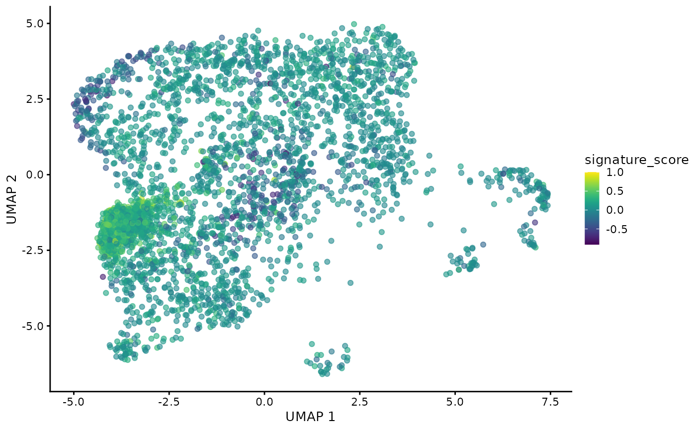

The cells could also be visualised using the popular and powerful ggplot2 package, enabling the researcher to use ggplot functions they were familiar with, and to customise the plot with great flexibility.

sce_obj |>
    
  join_features(
    features = c("CD3D", "TRDC", "TRGC1", "TRGC2", "CD8A", "CD8B"), shape = "wide"
  ) |>
    
  mutate(
    signature_score =
      scales::rescale(CD3D + TRDC + TRGC1 + TRGC2, to = c(0, 1)) -
        scales::rescale(CD8A + CD8B, to = c(0, 1))
  ) |>
    
  # plot cells with high score last so they're not obscured by other cells
  arrange(signature_score) |>
    
  ggplot(aes(UMAP_1, UMAP_2, color = signature_score)) +
  geom_point() +
  scale_color_distiller(palette = "Spectral") +
  bioc2022tidytranscriptomics::theme_multipanel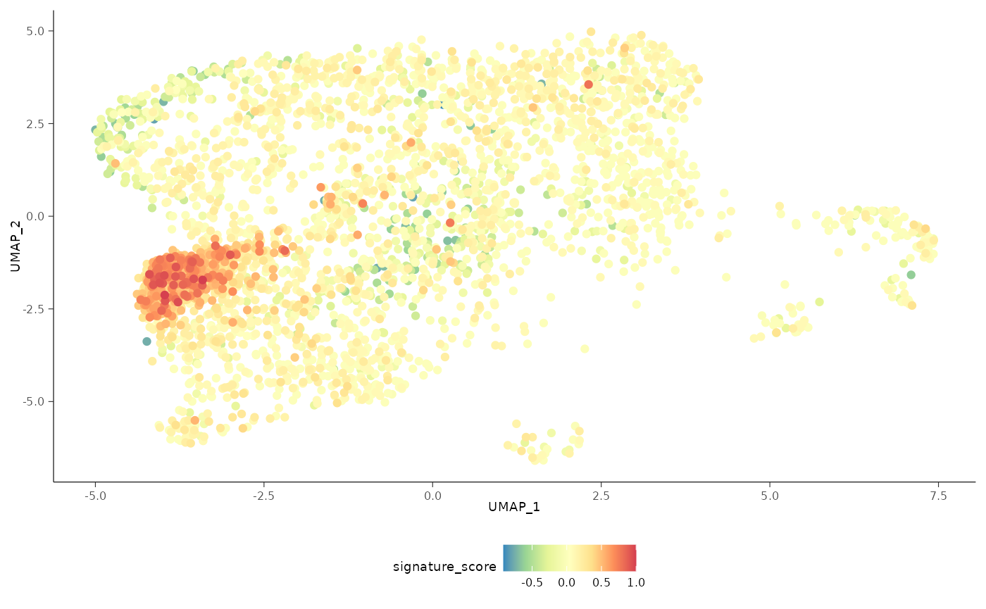

For exploratory analyses, we can select the gamma delta T cells, the red cluster on the left with high signature score. We’ll filter for cells with a signature score > 0.7.

sce_obj_gamma_delta <-
    
  sce_obj |>
    
  join_features(
    features = c("CD3D", "TRDC", "TRGC1", "TRGC2", "CD8A", "CD8B"), shape = "wide"
  ) |>
    
  mutate(
    signature_score =
      scales::rescale(CD3D + TRDC + TRGC1 + TRGC2, to = c(0, 1)) -
        scales::rescale(CD8A + CD8B, to = c(0, 1))
  ) |>
    
    # Proper cluster selection should be used instead (see supplementary material)
  filter(signature_score > 0.7)

For comparison, we show the alternative using base R and SingleCellExperiment. Note that the code contains more redundancy and intermediate objects.

counts_positive <-
  assay(sce_obj, "logcounts")[c("CD3D", "TRDC", "TRGC1", "TRGC2"), ] |>
  colSums() |>
  scales::rescale(to = c(0, 1))

counts_negative <-
  assay(sce_obj, "logcounts")[c("CD8A", "CD8B"), ] |>
  colSums() |>
  scales::rescale(to = c(0, 1))

sce_obj$signature_score <- counts_positive - counts_negative

sce_obj_gamma_delta <- sce_obj[, sce_obj$signature_score > 0.7]

We can then focus on just these gamma delta T cells and chain Bioconductor and tidyverse commands together to analyse.

library(batchelor)
library(scater)

sce_obj_gamma_delta <-
    
  sce_obj_gamma_delta |>
    
  # Integrate - using batchelor.
  multiBatchNorm(batch = colData(sce_obj_gamma_delta)$sample) |>
  fastMNN(batch = colData(sce_obj_gamma_delta)$sample) |>
    
  # Join metadata removed by fastMNN - using tidyverse
  left_join(as_tibble(sce_obj_gamma_delta)) |>
    
  # Dimension reduction - using scater
  runUMAP(ncomponents = 2, dimred = "corrected")

Visualise gamma delta T cells. As we have used rough threshold we are left with only few cells. Proper cluster selection should be used instead (see supplementary material).

sce_obj_gamma_delta |> plotUMAP()

It is also possible to visualise the cells as a 3D plot using plotly. The example data used here only contains a few genes, for the sake of time and size in this demonstration, but below is how you could generate the 3 dimensions needed for 3D plot with a full dataset.

single_cell_object |>
  RunUMAP(dims = 1:30, n.components = 3L, spread = 0.5, min.dist = 0.01, n.neighbors = 10L)

We’ll demonstrate creating a 3D plot using some data that has 3 UMAP dimensions. This is a fantastic way to visualise both reduced dimensions and metadata in the same representation.

pbmc <- bioc2022tidytranscriptomics::sce_obj_UMAP3

pbmc |>
  plot_ly(
    x = ~`UMAP_1`,
    y = ~`UMAP_2`,
    z = ~`UMAP_3`,
    color = ~cell_type,
    colors = dittoSeq::dittoColors()
  ) %>%
  add_markers(size = I(1))

Exercises

Using the sce_obj:

What proportion of all cells are gamma-delta T cells? Use signature_score > 0.7 to identify gamma-delta T cells.
There is a cluster of cells characterised by a low RNA output (nCount_RNA < 100). Identify the cell composition (cell_type) of that cluster.

Part 3 Pseudobulk analyses

Next we want to identify genes whose transcription is affected by treatment in this dataset, comparing treated and untreated patients. We can do this with pseudobulk analysis. We aggregate cell-wise transcript abundance into pseudobulk samples and can then perform hypothesis testing using the very well established bulk RNA sequencing tools. For example, we can use edgeR in tidybulk to perform differential expression testing. For more details on pseudobulk analysis see here.

We want to do it for each cell type and the tidy transcriptomics ecosystem makes this very easy.

Create pseudobulk samples

To create pseudobulk samples from the single cell samples, we will use a helper function called aggregate_cells, available in this workshop package. This function will combine the single cells into a group for each cell type for each sample.

pseudo_bulk <-
  sce_obj |>
  bioc2022tidytranscriptomics::aggregate_cells(c(sample, cell_type), assays = "counts")

pseudo_bulk

## # A SummarizedExperiment-tibble abstraction: 55,430 × 115
## # Features=482 | Samples=115 | Assays=counts
##    .feature   .sample    counts sample cell_…¹ .aggr…² batch sampl…³ BCB   file 
##    <chr>      <chr>       <dbl> <chr>  <fct>     <int> <fct> <chr>   <fct> <chr>
##  1 ABCC3      SI-GA-E5_…      0 SI-GA… CD4+_r…      24 2     SI-GA-… BCB0… ../d…
##  2 AC004585.1 SI-GA-E5_…      1 SI-GA… CD4+_r…      24 2     SI-GA-… BCB0… ../d…
##  3 AC005480.1 SI-GA-E5_…      0 SI-GA… CD4+_r…      24 2     SI-GA-… BCB0… ../d…
##  4 AC007952.4 SI-GA-E5_…      1 SI-GA… CD4+_r…      24 2     SI-GA-… BCB0… ../d…
##  5 AC012615.2 SI-GA-E5_…      0 SI-GA… CD4+_r…      24 2     SI-GA-… BCB0… ../d…
##  6 AC020656.1 SI-GA-E5_…      0 SI-GA… CD4+_r…      24 2     SI-GA-… BCB0… ../d…
##  7 AC021739.4 SI-GA-E5_…      0 SI-GA… CD4+_r…      24 2     SI-GA-… BCB0… ../d…
##  8 AC026979.2 SI-GA-E5_…      1 SI-GA… CD4+_r…      24 2     SI-GA-… BCB0… ../d…
##  9 AC046158.1 SI-GA-E5_…      0 SI-GA… CD4+_r…      24 2     SI-GA-… BCB0… ../d…
## 10 AC055713.1 SI-GA-E5_…      1 SI-GA… CD4+_r…      24 2     SI-GA-… BCB0… ../d…
## # … with 40 more rows, 2 more variables: treatment <chr>, feature <chr>, and
## #   abbreviated variable names ¹cell_type, ².aggregated_cells, ³sample_id
## # ℹ Use `print(n = ...)` to see more rows, and `colnames()` to see all variable names

Tidybulk and tidySummarizedExperiment

With tidySummarizedExperiment and tidybulk it is easy to split the data into groups and perform analyses on each without needing to create separate objects.

We use tidyverse nest to group the data. The command below will create a tibble containing a column with a SummarizedExperiment object for each cell type. nest is similar to tidyverse group_by, except with nest each group is stored in a single row, and can be a complex object such as a plot or SummarizedExperiment.

pseudo_bulk_nested <- 
  pseudo_bulk |>
  nest(grouped_summarized_experiment = -cell_type)

pseudo_bulk_nested

## # A tibble: 13 × 2
##    cell_type                                   grouped_summarized_experiment
##    <fct>                                       <list>                       
##  1 CD4+_ribosome_rich                          <SmmrzdEx[,10]>              
##  2 CD4+_Tcm_S100A4_IL32_IL7R_VIM               <SmmrzdEx[,10]>              
##  3 CD8+_high_ribonucleosome                    <SmmrzdEx[,10]>              
##  4 CD8+_Tcm                                    <SmmrzdEx[,6]>               
##  5 CD8+_transitional_effector_GZMK_KLRB1_LYAR4 <SmmrzdEx[,10]>              
##  6 HSC_lymphoid_myeloid_like                   <SmmrzdEx[,10]>              
##  7 limphoid_myeloid_like_HLA_CD74              <SmmrzdEx[,3]>               
##  8 MAIT                                        <SmmrzdEx[,10]>              
##  9 NK_cells                                    <SmmrzdEx[,10]>              
## 10 NK_cycling                                  <SmmrzdEx[,7]>               
## 11 T_cell:CD8+_other                           <SmmrzdEx[,10]>              
## 12 TCR_V_Delta_1                               <SmmrzdEx[,10]>              
## 13 TCR_V_Delta_2                               <SmmrzdEx[,9]>

To explore the grouping, we can use tidyverse slice to choose a row (cell_type) and pull to extract the values from a column. If we pull the data column we can view the SummarizedExperiment object.

pseudo_bulk_nested |>
  slice(1) |>
  pull(grouped_summarized_experiment)

## [[1]]
## # A SummarizedExperiment-tibble abstraction: 4,820 × 10
## # Features=482 | Samples=10 | Assays=counts
##    .feature   .sample    counts sample .aggr…¹ batch sampl…² BCB   file  treat…³
##    <chr>      <chr>       <dbl> <chr>    <int> <fct> <chr>   <fct> <chr> <chr>  
##  1 ABCC3      SI-GA-E5_…      0 SI-GA…      24 2     SI-GA-… BCB0… ../d… treated
##  2 AC004585.1 SI-GA-E5_…      1 SI-GA…      24 2     SI-GA-… BCB0… ../d… treated
##  3 AC005480.1 SI-GA-E5_…      0 SI-GA…      24 2     SI-GA-… BCB0… ../d… treated
##  4 AC007952.4 SI-GA-E5_…      1 SI-GA…      24 2     SI-GA-… BCB0… ../d… treated
##  5 AC012615.2 SI-GA-E5_…      0 SI-GA…      24 2     SI-GA-… BCB0… ../d… treated
##  6 AC020656.1 SI-GA-E5_…      0 SI-GA…      24 2     SI-GA-… BCB0… ../d… treated
##  7 AC021739.4 SI-GA-E5_…      0 SI-GA…      24 2     SI-GA-… BCB0… ../d… treated
##  8 AC026979.2 SI-GA-E5_…      1 SI-GA…      24 2     SI-GA-… BCB0… ../d… treated
##  9 AC046158.1 SI-GA-E5_…      0 SI-GA…      24 2     SI-GA-… BCB0… ../d… treated
## 10 AC055713.1 SI-GA-E5_…      1 SI-GA…      24 2     SI-GA-… BCB0… ../d… treated
## # … with 40 more rows, 1 more variable: feature <chr>, and abbreviated variable
## #   names ¹.aggregated_cells, ²sample_id, ³treatment
## # ℹ Use `print(n = ...)` to see more rows, and `colnames()` to see all variable names

We can then identify differentially expressed genes for each cell type for our condition of interest, treated versus untreated patients. We use tidyverse map to apply differential expression functions to each cell type group in the nested data. The result columns will be added to the SummarizedExperiment objects.

# Differential transcription abundance
pseudo_bulk <-
    
  pseudo_bulk_nested |>
    
  # map accepts a data column (.x) and a function. It applies the function to each element of the column.
  mutate(grouped_summarized_experiment = map(
    grouped_summarized_experiment,
    ~ .x |>
        
      # Removing genes with low expression
      identify_abundant(factor_of_interest = treatment) |>
        
      # Scaling counts for sequencing depth 
      scale_abundance(method="TMMwsp") |>
      
      # Testing for differential expression using edgeR quasi likelihood    
      test_differential_abundance(~treatment, method="edgeR_quasi_likelihood", scaling_method="TMMwsp")
  ))

The output is again a tibble containing a SummarizedExperiment object for each cell type.

pseudo_bulk

## # A tibble: 13 × 2
##    cell_type                                   grouped_summarized_experiment
##    <fct>                                       <list>                       
##  1 CD4+_ribosome_rich                          <SmmrzdEx[,10]>              
##  2 CD4+_Tcm_S100A4_IL32_IL7R_VIM               <SmmrzdEx[,10]>              
##  3 CD8+_high_ribonucleosome                    <SmmrzdEx[,10]>              
##  4 CD8+_Tcm                                    <SmmrzdEx[,6]>               
##  5 CD8+_transitional_effector_GZMK_KLRB1_LYAR4 <SmmrzdEx[,10]>              
##  6 HSC_lymphoid_myeloid_like                   <SmmrzdEx[,10]>              
##  7 limphoid_myeloid_like_HLA_CD74              <SmmrzdEx[,3]>               
##  8 MAIT                                        <SmmrzdEx[,10]>              
##  9 NK_cells                                    <SmmrzdEx[,10]>              
## 10 NK_cycling                                  <SmmrzdEx[,7]>               
## 11 T_cell:CD8+_other                           <SmmrzdEx[,10]>              
## 12 TCR_V_Delta_1                               <SmmrzdEx[,10]>              
## 13 TCR_V_Delta_2                               <SmmrzdEx[,9]>

If we pull out the SummarizedExperiment object for the first cell type, as before, we can see it now has columns containing the differential expression results (e.g. logFC, PValue).

pseudo_bulk |>
  slice(1) |>
  pull(grouped_summarized_experiment)

## [[1]]
## # A SummarizedExperiment-tibble abstraction: 4,820 × 10
## # Features=482 | Samples=10 | Assays=counts, counts_scaled
##    .feature   .sample    counts count…¹ sample .aggr…² batch sampl…³ BCB   file 
##    <chr>      <chr>       <dbl>   <dbl> <chr>    <int> <fct> <chr>   <fct> <chr>
##  1 ABCC3      SI-GA-E5_…      0    0    SI-GA…      24 2     SI-GA-… BCB0… ../d…
##  2 AC004585.1 SI-GA-E5_…      1    6.12 SI-GA…      24 2     SI-GA-… BCB0… ../d…
##  3 AC005480.1 SI-GA-E5_…      0    0    SI-GA…      24 2     SI-GA-… BCB0… ../d…
##  4 AC007952.4 SI-GA-E5_…      1    6.12 SI-GA…      24 2     SI-GA-… BCB0… ../d…
##  5 AC012615.2 SI-GA-E5_…      0    0    SI-GA…      24 2     SI-GA-… BCB0… ../d…
##  6 AC020656.1 SI-GA-E5_…      0    0    SI-GA…      24 2     SI-GA-… BCB0… ../d…
##  7 AC021739.4 SI-GA-E5_…      0    0    SI-GA…      24 2     SI-GA-… BCB0… ../d…
##  8 AC026979.2 SI-GA-E5_…      1    6.12 SI-GA…      24 2     SI-GA-… BCB0… ../d…
##  9 AC046158.1 SI-GA-E5_…      0    0    SI-GA…      24 2     SI-GA-… BCB0… ../d…
## 10 AC055713.1 SI-GA-E5_…      1    6.12 SI-GA…      24 2     SI-GA-… BCB0… ../d…
## # … with 40 more rows, 10 more variables: treatment <chr>, TMM <dbl>,
## #   multiplier <dbl>, feature <chr>, .abundant <lgl>, logFC <dbl>,
## #   logCPM <dbl>, F <dbl>, PValue <dbl>, FDR <dbl>, and abbreviated variable
## #   names ¹counts_scaled, ².aggregated_cells, ³sample_id
## # ℹ Use `print(n = ...)` to see more rows, and `colnames()` to see all variable names

It is useful to create plots for significant genes to visualise the transcriptional abundance in the groups being compared (treated and untreated). We can do this for each cell type without needing to create multiple objects.

pseudo_bulk <-
    
  pseudo_bulk |>
    
  # Filter out significant
  # using a high FDR value as this is toy data
  mutate(grouped_summarized_experiment = map(
    grouped_summarized_experiment, 
    ~ filter(.x, FDR < 0.5)
  )) |>
    
  # Filter cell types with no differential abundant gene-transcripts
  # map_int is map that returns integer instead of list
  filter(map_int(grouped_summarized_experiment, ~ nrow(.x)) > 0) |>

  # Plot significant genes for each cell type
  # map2 is map that accepts 2 input columns (.x, .y) and a function
  mutate(plot = map2(
    grouped_summarized_experiment, cell_type,
    ~ .x |>
      ggplot(aes(treatment, counts_scaled + 1)) +
      geom_boxplot(aes(fill = treatment)) +
      geom_jitter() +
      scale_y_log10() +
      facet_wrap(~.feature) +
      ggtitle(.y)
  ))

The output is a nested table with a column containing a plot for each cell type.

pseudo_bulk

## # A tibble: 5 × 3
##   cell_type                      grouped_summarized_experiment plot  
##   <fct>                          <list>                        <list>
## 1 CD4+_ribosome_rich             <SmmrzdEx[,10]>               <gg>  
## 2 limphoid_myeloid_like_HLA_CD74 <SmmrzdEx[,3]>                <gg>  
## 3 NK_cells                       <SmmrzdEx[,10]>               <gg>  
## 4 T_cell:CD8+_other              <SmmrzdEx[,10]>               <gg>  
## 5 TCR_V_Delta_1                  <SmmrzdEx[,10]>               <gg>

We’ll use slice and pull again to have a look at one of the plots.

pseudo_bulk |>
  slice(1) |>
  pull(plot)

## [[1]]

We can extract all plots and plot with wrap_plots from the patchwork package.

pseudo_bulk |>
  pull(plot) |>
  wrap_plots() &
  bioc2022tidytranscriptomics::theme_multipanel

Feedback

Thank you for attending this workshop. We hope it was an informative session for you. We would be grateful if you could help us by taking a few moments to provide your valuable feedback in the short form below. Your feedback will provide us with an opportunity to further improve the workshop. All the results are anonymous.

Feedback Form Link

Session Information

sessionInfo()

## R version 4.2.0 (2022-04-22)
## Platform: x86_64-pc-linux-gnu (64-bit)
## Running under: Ubuntu 20.04.4 LTS
## 
## Matrix products: default
## BLAS:   /usr/lib/x86_64-linux-gnu/openblas-pthread/libblas.so.3
## LAPACK: /usr/lib/x86_64-linux-gnu/openblas-pthread/liblapack.so.3
## 
## locale:
##  [1] LC_CTYPE=en_US.UTF-8       LC_NUMERIC=C              
##  [3] LC_TIME=en_US.UTF-8        LC_COLLATE=en_US.UTF-8    
##  [5] LC_MONETARY=en_US.UTF-8    LC_MESSAGES=en_US.UTF-8   
##  [7] LC_PAPER=en_US.UTF-8       LC_NAME=C                 
##  [9] LC_ADDRESS=C               LC_TELEPHONE=C            
## [11] LC_MEASUREMENT=en_US.UTF-8 LC_IDENTIFICATION=C       
## 
## attached base packages:
## [1] stats4    stats     graphics  grDevices utils     datasets  methods  
## [8] base     
## 
## other attached packages:
##  [1] tidySummarizedExperiment_1.7.3 tidybulk_1.9.2                
##  [3] patchwork_1.1.1                purrr_0.3.4                   
##  [5] tidyr_1.2.0                    glue_1.6.2                    
##  [7] scater_1.25.2                  scuttle_1.7.2                 
##  [9] batchelor_1.13.3               tidySingleCellExperiment_1.7.4
## [11] ttservice_0.2.2                dittoSeq_1.9.1                
## [13] colorspace_2.0-3               dplyr_1.0.9                   
## [15] plotly_4.10.0                  ggplot2_3.3.6                 
## [17] SingleCellExperiment_1.19.0    SummarizedExperiment_1.27.1   
## [19] Biobase_2.57.1                 GenomicRanges_1.49.0          
## [21] GenomeInfoDb_1.33.3            IRanges_2.31.0                
## [23] S4Vectors_0.35.1               BiocGenerics_0.43.1           
## [25] MatrixGenerics_1.9.1           matrixStats_0.62.0            
## 
## loaded via a namespace (and not attached):
##   [1] ggbeeswarm_0.6.0                   ellipsis_0.3.2                    
##   [3] bioc2022tidytranscriptomics_0.13.3 ggridges_0.5.3                    
##   [5] rprojroot_2.0.3                    XVector_0.37.0                    
##   [7] BiocNeighbors_1.15.1               fs_1.5.2                          
##   [9] farver_2.1.1                       ggrepel_0.9.1                     
##  [11] RSpectra_0.16-1                    fansi_1.0.3                       
##  [13] splines_4.2.0                      codetools_0.2-18                  
##  [15] sparseMatrixStats_1.9.0            cachem_1.0.6                      
##  [17] knitr_1.39                         jsonlite_1.8.0                    
##  [19] ResidualMatrix_1.7.0               pheatmap_1.0.12                   
##  [21] uwot_0.1.11                        BiocManager_1.30.18               
##  [23] readr_2.1.2                        compiler_4.2.0                    
##  [25] httr_1.4.3                         Matrix_1.4-1                      
##  [27] fastmap_1.1.0                      lazyeval_0.2.2                    
##  [29] limma_3.53.5                       cli_3.3.0                         
##  [31] BiocSingular_1.13.0                htmltools_0.5.3                   
##  [33] tools_4.2.0                        rsvd_1.0.5                        
##  [35] igraph_1.3.4                       gtable_0.3.0                      
##  [37] GenomeInfoDbData_1.2.8             Rcpp_1.0.9                        
##  [39] jquerylib_0.1.4                    pkgdown_2.0.6                     
##  [41] vctrs_0.4.1                        preprocessCore_1.59.0             
##  [43] crosstalk_1.2.0                    DelayedMatrixStats_1.19.0         
##  [45] xfun_0.31                          stringr_1.4.0                     
##  [47] beachmat_2.13.4                    lifecycle_1.0.1                   
##  [49] irlba_2.3.5                        edgeR_3.39.3                      
##  [51] zlibbioc_1.43.0                    scales_1.2.0                      
##  [53] ragg_1.2.2                         hms_1.1.1                         
##  [55] parallel_4.2.0                     RColorBrewer_1.1-3                
##  [57] yaml_2.3.5                         memoise_2.0.1                     
##  [59] gridExtra_2.3                      sass_0.4.2                        
##  [61] stringi_1.7.8                      highr_0.9                         
##  [63] desc_1.4.1                         ScaledMatrix_1.5.0                
##  [65] BiocParallel_1.31.10               rlang_1.0.4                       
##  [67] pkgconfig_2.0.3                    systemfonts_1.0.4                 
##  [69] bitops_1.0-7                       evaluate_0.15                     
##  [71] lattice_0.20-45                    htmlwidgets_1.5.4                 
##  [73] labeling_0.4.2                     cowplot_1.1.1                     
##  [75] tidyselect_1.1.2                   plyr_1.8.7                        
##  [77] magrittr_2.0.3                     R6_2.5.1                          
##  [79] generics_0.1.3                     DelayedArray_0.23.0               
##  [81] pillar_1.8.0                       withr_2.5.0                       
##  [83] RCurl_1.98-1.7                     tibble_3.1.8                      
##  [85] crayon_1.5.1                       utf8_1.2.2                        
##  [87] tzdb_0.3.0                         rmarkdown_2.14                    
##  [89] viridis_0.6.2                      locfit_1.5-9.5                    
##  [91] grid_4.2.0                         data.table_1.14.2                 
##  [93] FNN_1.1.3.1                        digest_0.6.29                     
##  [95] textshaping_0.3.6                  munsell_0.5.0                     
##  [97] beeswarm_0.4.0                     viridisLite_0.4.0                 
##  [99] vipor_0.4.5                        bslib_0.4.0

References

Butler, Andrew, Paul Hoffman, Peter Smibert, Efthymia Papalexi, and Rahul Satija. 2018. “Integrating Single-Cell Transcriptomic Data Across Different Conditions, Technologies, and Species.” Nature Biotechnology 36 (5): 411–20.

Pizzolato, Gabriele, Hannah Kaminski, Marie Tosolini, Don-Marc Franchini, Fréderic Pont, Fréderic Martins, Carine Valle, et al. 2019. “Single-Cell RNA Sequencing Unveils the Shared and the Distinct Cytotoxic Hallmarks of Human TCRV\(\updelta\)1 and TCRV\(\updelta\)2 \(\upgamma\)\(\updelta\) t Lymphocytes.” Proceedings of the National Academy of Sciences, May, 201818488. https://doi.org/10.1073/pnas.1818488116.

Stuart, Tim, Andrew Butler, Paul Hoffman, Christoph Hafemeister, Efthymia Papalexi, William M Mauck III, Yuhan Hao, Marlon Stoeckius, Peter Smibert, and Rahul Satija. 2019. “Comprehensive Integration of Single-Cell Data.” Cell 177 (7): 1888–1902.

Wickham, Hadley, Mara Averick, Jennifer Bryan, Winston Chang, Lucy D’Agostino McGowan, Romain François, Garrett Grolemund, et al. 2019. “Welcome to the Tidyverse.” Journal of Open Source Software 4 (43): 1686.

<mangiola.s at wehi.edu.au>↩︎
<maria.doyle at petermac.org>↩︎

Stefano Mangiola, Walter and Eliza Hall Institute¹

Maria Doyle, Peter MacCallum Cancer Centre²

Workshop introduction

Instructors

Description

Pre-requisites

Goals and objectives

What you will learn

What you will not learn

Getting started

Cloud

Local

Slides

Part 1 Introduction to tidySingleCellExperiment

Tidyverse commands

Part 2 Signature visualisation

Data pre-processing

Analyse custom signature

Exercises

Part 3 Pseudobulk analyses

Create pseudobulk samples

Tidybulk and tidySummarizedExperiment

Feedback

Tidy Transcriptomics For Single-Cell RNA Sequencing Analyses

Stefano Mangiola, Walter and Eliza Hall Institute1

Maria Doyle, Peter MacCallum Cancer Centre2

Workshop introduction

Instructors

Description

Pre-requisites

Goals and objectives

What you will learn

What you will not learn

Getting started

Cloud

Local

Slides

Part 1 Introduction to tidySingleCellExperiment

Tidyverse commands

Part 2 Signature visualisation

Data pre-processing

Analyse custom signature

Exercises

Part 3 Pseudobulk analyses

Create pseudobulk samples

Tidybulk and tidySummarizedExperiment

Feedback

Stefano Mangiola, Walter and Eliza Hall Institute¹

Maria Doyle, Peter MacCallum Cancer Centre²