Tidy Transcriptomics for Single-cell RNA Sequencing Analyses

Instructors

Dr. Stefano Mangiola is currently a Postdoctoral researcher in the laboratory of Prof. Tony Papenfuss at the Walter and Eliza Hall Institute in Melbourne, Australia. His background spans from biotechnology to bioinformatics and biostatistics. His research focuses on prostate and breast tumour microenvironment, the development of statistical models for the analysis of RNA sequencing data, and data analysis and visualisation interfaces.

Workshop goals and objectives

What you will learn

Basic tidy operations possible with tidyseurat and tidySingleCellExperiment
The differences between Seurat and SingleCellExperiment representation, and tidy representation
How to interface Seurat and SingleCellExperiment with tidy manipulation and visualisation
A real-world case study that will showcase the power of tidy single-cell methods compared with base/ad-hoc methods

What you will not learn

The molecular technology of single-cell sequencing
The fundamentals of single-cell data analysis
The fundamentals of tidy data analysis

Getting started

Local

We will use the Cloud during the workshop and this method is available if you want to run the material after the workshop. If you want to install on your own computer, see instructions here.

Alternatively, you can view the material at the workshop webpage here.

Introduction to tidytranscriptomics

Here

Part 1 Introduction to tidyseurat

# Load packages
library(purrr)
library(Seurat)
library(ggplot2)
library(dplyr)
library(colorspace)
library(dittoSeq)

Seurat is a very popular analysis toolkit for single cell RNA sequencing data (Butler et al. 2018; Stuart et al. 2019).

Here we load single-cell data in Seurat object format. This data is peripheral blood mononuclear cells (PBMCs) from metastatic breast cancer patients.

# load single cell RNA sequencing data
seurat_obj <- RMedicine2023tidytranscriptomics::seurat_obj

# take a look
seurat_obj

## An object of class Seurat 
## 3006 features across 33215 samples within 2 assays 
## Active assay: SCT (6 features, 0 variable features)
##  1 other assay present: RNA
##  1 dimensional reduction calculated: umap

tidyseurat provides a bridge between the Seurat single-cell package and the tidyverse (Wickham et al. 2019). It creates an invisible layer that enables viewing the Seurat object as a tidyverse tibble, and provides Seurat-compatible dplyr, tidyr, ggplot and plotly functions.

If we load the tidyseurat package and then view the single cell data, it now displays as a tibble.

library(tidyseurat)

seurat_obj

## # A Seurat-tibble abstraction: 33,215 × 18
## # Features=6 | Cells=33215 | Active assay=SCT | Assays=RNA, SCT
##    .cell      file  sample_id sample Barcode batch BCB   S.Score G2M.Score Phase
##    <chr>      <chr> <chr>     <chr>  <chr>   <chr> <chr>   <dbl>     <dbl> <chr>
##  1 1_AAACGAA… ../d… SI-GA-H1… SI-GA… AAACGA… 1     BCB1…  0.0620   -0.0972 S    
##  2 1_AAACGCT… ../d… SI-GA-H1… SI-GA… AAACGC… 1     BCB1…  0.0943   -0.193  S    
##  3 1_AAACGCT… ../d… SI-GA-H1… SI-GA… AAACGC… 1     BCB1…  0.0216   -0.124  S    
##  4 1_AAAGAAC… ../d… SI-GA-H1… SI-GA… AAAGAA… 1     BCB1…  0.0598   -0.196  S    
##  5 1_AAAGGAT… ../d… SI-GA-H1… SI-GA… AAAGGA… 1     BCB1…  0.0281   -0.0540 S    
##  6 1_AAAGGGC… ../d… SI-GA-H1… SI-GA… AAAGGG… 1     BCB1…  0.0110   -0.0998 S    
##  7 1_AAAGGGC… ../d… SI-GA-H1… SI-GA… AAAGGG… 1     BCB1…  0.0341   -0.143  S    
##  8 1_AAAGTCC… ../d… SI-GA-H1… SI-GA… AAAGTC… 1     BCB1…  0.0425   -0.183  S    
##  9 1_AAAGTCC… ../d… SI-GA-H1… SI-GA… AAAGTC… 1     BCB1… -0.0289   -0.127  G1   
## 10 1_AAAGTGA… ../d… SI-GA-H1… SI-GA… AAAGTG… 1     BCB1… -0.0551   -0.102  G1   
## # ℹ 33,205 more rows
## # ℹ 8 more variables: curated_cell_type <chr>, nCount_RNA <dbl>,
## #   nFeature_RNA <int>, nCount_SCT <dbl>, nFeature_SCT <int>, treatment <fct>,
## #   UMAP_1 <dbl>, UMAP_2 <dbl>

If we want to revert to the standard SingleCellExperiment view we can do that.

options("restore_Seurat_show" = TRUE)
seurat_obj

## An object of class Seurat 
## 3006 features across 33215 samples within 2 assays 
## Active assay: SCT (6 features, 0 variable features)
##  1 other assay present: RNA
##  1 dimensional reduction calculated: umap

If we want to revert back to tidy SingleCellExperiment view we can.

options("restore_Seurat_show" = FALSE)
seurat_obj

## # A Seurat-tibble abstraction: 33,215 × 18
## # Features=6 | Cells=33215 | Active assay=SCT | Assays=RNA, SCT
##    .cell      file  sample_id sample Barcode batch BCB   S.Score G2M.Score Phase
##    <chr>      <chr> <chr>     <chr>  <chr>   <chr> <chr>   <dbl>     <dbl> <chr>
##  1 1_AAACGAA… ../d… SI-GA-H1… SI-GA… AAACGA… 1     BCB1…  0.0620   -0.0972 S    
##  2 1_AAACGCT… ../d… SI-GA-H1… SI-GA… AAACGC… 1     BCB1…  0.0943   -0.193  S    
##  3 1_AAACGCT… ../d… SI-GA-H1… SI-GA… AAACGC… 1     BCB1…  0.0216   -0.124  S    
##  4 1_AAAGAAC… ../d… SI-GA-H1… SI-GA… AAAGAA… 1     BCB1…  0.0598   -0.196  S    
##  5 1_AAAGGAT… ../d… SI-GA-H1… SI-GA… AAAGGA… 1     BCB1…  0.0281   -0.0540 S    
##  6 1_AAAGGGC… ../d… SI-GA-H1… SI-GA… AAAGGG… 1     BCB1…  0.0110   -0.0998 S    
##  7 1_AAAGGGC… ../d… SI-GA-H1… SI-GA… AAAGGG… 1     BCB1…  0.0341   -0.143  S    
##  8 1_AAAGTCC… ../d… SI-GA-H1… SI-GA… AAAGTC… 1     BCB1…  0.0425   -0.183  S    
##  9 1_AAAGTCC… ../d… SI-GA-H1… SI-GA… AAAGTC… 1     BCB1… -0.0289   -0.127  G1   
## 10 1_AAAGTGA… ../d… SI-GA-H1… SI-GA… AAAGTG… 1     BCB1… -0.0551   -0.102  G1   
## # ℹ 33,205 more rows
## # ℹ 8 more variables: curated_cell_type <chr>, nCount_RNA <dbl>,
## #   nFeature_RNA <int>, nCount_SCT <dbl>, nFeature_SCT <int>, treatment <fct>,
## #   UMAP_1 <dbl>, UMAP_2 <dbl>

It can be interacted with using Seurat commands such as Assays.

Assays(seurat_obj)

## [1] "RNA" "SCT"

We can also interact with our object as we do with any tidyverse tibble.

Tidyverse commands

We can use tidyverse commands, such as filter, select and mutate to explore the tidyseurat object. Some examples are shown below and more can be seen at the tidyseurat website here.

We can use filter to choose rows, for example, to see just the rows for the cells in G1 cell-cycle stage. Check if have groups or ident present.

seurat_obj |> filter(Phase == "G1")

## # A Seurat-tibble abstraction: 18,141 × 18
## # Features=6 | Cells=18141 | Active assay=SCT | Assays=RNA, SCT
##    .cell     file  sample_id sample Barcode batch BCB    S.Score G2M.Score Phase
##    <chr>     <chr> <chr>     <chr>  <chr>   <chr> <chr>    <dbl>     <dbl> <chr>
##  1 1_AAAGTC… ../d… SI-GA-H1… SI-GA… AAAGTC… 1     BCB1… -0.0289   -0.127   G1   
##  2 1_AAAGTG… ../d… SI-GA-H1… SI-GA… AAAGTG… 1     BCB1… -0.0551   -0.102   G1   
##  3 1_AAATGG… ../d… SI-GA-H1… SI-GA… AAATGG… 1     BCB1… -0.0207   -0.0602  G1   
##  4 1_AAATGG… ../d… SI-GA-H1… SI-GA… AAATGG… 1     BCB1… -0.0195   -0.00881 G1   
##  5 1_AACAAC… ../d… SI-GA-H1… SI-GA… AACAAC… 1     BCB1… -0.0421   -0.197   G1   
##  6 1_AACAAC… ../d… SI-GA-H1… SI-GA… AACAAC… 1     BCB1… -0.0105   -0.0902  G1   
##  7 1_AACACA… ../d… SI-GA-H1… SI-GA… AACACA… 1     BCB1… -0.0164   -0.132   G1   
##  8 1_AACAGG… ../d… SI-GA-H1… SI-GA… AACAGG… 1     BCB1… -0.00158  -0.0652  G1   
##  9 1_AACCAA… ../d… SI-GA-H1… SI-GA… AACCAA… 1     BCB1… -0.00504  -0.135   G1   
## 10 1_AACGGG… ../d… SI-GA-H1… SI-GA… AACGGG… 1     BCB1… -0.00701  -0.0919  G1   
## # ℹ 18,131 more rows
## # ℹ 8 more variables: curated_cell_type <chr>, nCount_RNA <dbl>,
## #   nFeature_RNA <int>, nCount_SCT <dbl>, nFeature_SCT <int>, treatment <fct>,
## #   UMAP_1 <dbl>, UMAP_2 <dbl>

We can use select to choose columns, for example, to see the sample, cell, total cellular RNA

seurat_obj |> select(.cell, nCount_RNA, Phase)

## # A Seurat-tibble abstraction: 33,215 × 5
## # Features=6 | Cells=33215 | Active assay=SCT | Assays=RNA, SCT
##    .cell                nCount_RNA Phase UMAP_1 UMAP_2
##    <chr>                     <dbl> <chr>  <dbl>  <dbl>
##  1 1_AAACGAACAAAGGCAC-1       1485 S       2.56 -2.99 
##  2 1_AAACGCTCATGAATAG-1       2460 S      -3.32 -3.84 
##  3 1_AAACGCTTCTTGGATG-1       1739 S       2.51 -3.15 
##  4 1_AAAGAACCAACGGCTC-1       2346 S      -3.11 -0.166
##  5 1_AAAGGATTCCCGTTCA-1        763 S      -3.50 -0.754
##  6 1_AAAGGGCAGGCATTTC-1       2001 S       1.54 -2.10 
##  7 1_AAAGGGCCAGAGATTA-1       1907 S      -3.20 -1.92 
##  8 1_AAAGTCCAGTAACGAT-1       2239 S      -4.03  0.347
##  9 1_AAAGTCCGTAATTAGG-1       1697 G1     -3.24 -3.48 
## 10 1_AAAGTGAGTATGGGAC-1       2374 G1     -2.03 -3.56 
## # ℹ 33,205 more rows

We also see the UMAP columns as they are not part of the cell metadata, they are read-only. If we want to save the edited metadata, the Seurat object is modified accordingly.

# Save edited metadata
seurat_modified <- seurat_obj |> select(.cell, nCount_RNA, Phase)
# View Seurat metadata
seurat_modified[[]] |> head()

##                      nCount_RNA Phase
## 1_AAACGAACAAAGGCAC-1       1485     S
## 1_AAACGCTCATGAATAG-1       2460     S
## 1_AAACGCTTCTTGGATG-1       1739     S
## 1_AAAGAACCAACGGCTC-1       2346     S
## 1_AAAGGATTCCCGTTCA-1        763     S
## 1_AAAGGGCAGGCATTTC-1       2001     S

We can use mutate to create a column. For example, we could create a new Phase_l column that contains a lower-case version of Phase.

seurat_obj |>
    mutate(Phase_l=tolower(Phase)) |>
    
    # Select columns to view    
    select(.cell, Phase, Phase_l)

## # A Seurat-tibble abstraction: 33,215 × 5
## # Features=6 | Cells=33215 | Active assay=SCT | Assays=RNA, SCT
##    .cell                Phase Phase_l UMAP_1 UMAP_2
##    <chr>                <chr> <chr>    <dbl>  <dbl>
##  1 1_AAACGAACAAAGGCAC-1 S     s         2.56 -2.99 
##  2 1_AAACGCTCATGAATAG-1 S     s        -3.32 -3.84 
##  3 1_AAACGCTTCTTGGATG-1 S     s         2.51 -3.15 
##  4 1_AAAGAACCAACGGCTC-1 S     s        -3.11 -0.166
##  5 1_AAAGGATTCCCGTTCA-1 S     s        -3.50 -0.754
##  6 1_AAAGGGCAGGCATTTC-1 S     s         1.54 -2.10 
##  7 1_AAAGGGCCAGAGATTA-1 S     s        -3.20 -1.92 
##  8 1_AAAGTCCAGTAACGAT-1 S     s        -4.03  0.347
##  9 1_AAAGTCCGTAATTAGG-1 G1    g1       -3.24 -3.48 
## 10 1_AAAGTGAGTATGGGAC-1 G1    g1       -2.03 -3.56 
## # ℹ 33,205 more rows

We can use tidyverse commands to polish an annotation column. We will extract the sample, and group information from the file name column into separate columns.

# First take a look at the file column
seurat_obj |> select(.cell, file)

## # A Seurat-tibble abstraction: 33,215 × 4
## # Features=6 | Cells=33215 | Active assay=SCT | Assays=RNA, SCT
##    .cell                file                                       UMAP_1 UMAP_2
##    <chr>                <chr>                                       <dbl>  <dbl>
##  1 1_AAACGAACAAAGGCAC-1 ../data/experiment_10X_260819/SI-GA-H1/ou…   2.56 -2.99 
##  2 1_AAACGCTCATGAATAG-1 ../data/experiment_10X_260819/SI-GA-H1/ou…  -3.32 -3.84 
##  3 1_AAACGCTTCTTGGATG-1 ../data/experiment_10X_260819/SI-GA-H1/ou…   2.51 -3.15 
##  4 1_AAAGAACCAACGGCTC-1 ../data/experiment_10X_260819/SI-GA-H1/ou…  -3.11 -0.166
##  5 1_AAAGGATTCCCGTTCA-1 ../data/experiment_10X_260819/SI-GA-H1/ou…  -3.50 -0.754
##  6 1_AAAGGGCAGGCATTTC-1 ../data/experiment_10X_260819/SI-GA-H1/ou…   1.54 -2.10 
##  7 1_AAAGGGCCAGAGATTA-1 ../data/experiment_10X_260819/SI-GA-H1/ou…  -3.20 -1.92 
##  8 1_AAAGTCCAGTAACGAT-1 ../data/experiment_10X_260819/SI-GA-H1/ou…  -4.03  0.347
##  9 1_AAAGTCCGTAATTAGG-1 ../data/experiment_10X_260819/SI-GA-H1/ou…  -3.24 -3.48 
## 10 1_AAAGTGAGTATGGGAC-1 ../data/experiment_10X_260819/SI-GA-H1/ou…  -2.03 -3.56 
## # ℹ 33,205 more rows

# Create columns for sample and group
seurat_obj <- seurat_obj |>
    
    # Extract sample and group
    extract(file, "sample", "../data/.*/([a-zA-Z0-9_-]+)/outs.+", remove = FALSE)

# Take a look
seurat_obj |> select(.cell, sample)

## # A Seurat-tibble abstraction: 33,215 × 4
## # Features=6 | Cells=33215 | Active assay=SCT | Assays=RNA, SCT
##    .cell                sample   UMAP_1 UMAP_2
##    <chr>                <chr>     <dbl>  <dbl>
##  1 1_AAACGAACAAAGGCAC-1 SI-GA-H1   2.56 -2.99 
##  2 1_AAACGCTCATGAATAG-1 SI-GA-H1  -3.32 -3.84 
##  3 1_AAACGCTTCTTGGATG-1 SI-GA-H1   2.51 -3.15 
##  4 1_AAAGAACCAACGGCTC-1 SI-GA-H1  -3.11 -0.166
##  5 1_AAAGGATTCCCGTTCA-1 SI-GA-H1  -3.50 -0.754
##  6 1_AAAGGGCAGGCATTTC-1 SI-GA-H1   1.54 -2.10 
##  7 1_AAAGGGCCAGAGATTA-1 SI-GA-H1  -3.20 -1.92 
##  8 1_AAAGTCCAGTAACGAT-1 SI-GA-H1  -4.03  0.347
##  9 1_AAAGTCCGTAATTAGG-1 SI-GA-H1  -3.24 -3.48 
## 10 1_AAAGTGAGTATGGGAC-1 SI-GA-H1  -2.03 -3.56 
## # ℹ 33,205 more rows

We could use tidyverse unite to combine columns, for example to create a new column for sample id that combines the sample and patient identifier (BCB) columns.

seurat_obj <- seurat_obj |> unite("sample_id", sample, BCB, remove = FALSE)

# Take a look
seurat_obj |> select(.cell, sample_id, sample, BCB)

## # A Seurat-tibble abstraction: 33,215 × 6
## # Features=6 | Cells=33215 | Active assay=SCT | Assays=RNA, SCT
##    .cell                sample_id       sample   BCB    UMAP_1 UMAP_2
##    <chr>                <chr>           <chr>    <chr>   <dbl>  <dbl>
##  1 1_AAACGAACAAAGGCAC-1 SI-GA-H1_BCB102 SI-GA-H1 BCB102   2.56 -2.99 
##  2 1_AAACGCTCATGAATAG-1 SI-GA-H1_BCB102 SI-GA-H1 BCB102  -3.32 -3.84 
##  3 1_AAACGCTTCTTGGATG-1 SI-GA-H1_BCB102 SI-GA-H1 BCB102   2.51 -3.15 
##  4 1_AAAGAACCAACGGCTC-1 SI-GA-H1_BCB102 SI-GA-H1 BCB102  -3.11 -0.166
##  5 1_AAAGGATTCCCGTTCA-1 SI-GA-H1_BCB102 SI-GA-H1 BCB102  -3.50 -0.754
##  6 1_AAAGGGCAGGCATTTC-1 SI-GA-H1_BCB102 SI-GA-H1 BCB102   1.54 -2.10 
##  7 1_AAAGGGCCAGAGATTA-1 SI-GA-H1_BCB102 SI-GA-H1 BCB102  -3.20 -1.92 
##  8 1_AAAGTCCAGTAACGAT-1 SI-GA-H1_BCB102 SI-GA-H1 BCB102  -4.03  0.347
##  9 1_AAAGTCCGTAATTAGG-1 SI-GA-H1_BCB102 SI-GA-H1 BCB102  -3.24 -3.48 
## 10 1_AAAGTGAGTATGGGAC-1 SI-GA-H1_BCB102 SI-GA-H1 BCB102  -2.03 -3.56 
## # ℹ 33,205 more rows

Part 2 Signature visualisation

We will now demonstrate a real-world example of the power of using tidy transcriptomics packages in single cell analysis. For more information on single-cell analysis steps performed in a tidy way please see the ISMB2021 workshop.

Data pre-processing

The object seurat_obj we’ve been using was created as part of a study on breast cancer systemic immune response. Peripheral blood mononuclear cells have been sequenced for RNA at the single-cell level. The steps used to generate the object are summarised below.

scran, scater, and DropletsUtils packages have been used to eliminate empty droplets and dead cells. Samples were individually quality checked and cells were filtered for good gene coverage.
Variable features were identified using Seurat.
Read counts were scaled and normalised using SCTtransform from Seurat.
Data integration was performed using Seurat with default parameters.
PCA performed to reduce feature dimensionality.
Nearest-neighbor cell networks were calculated using 30 principal components.
2 UMAP dimensions were calculated using 30 principal components.
Cells with similar transcriptome profiles were grouped into clusters using Louvain clustering from Seurat.

Analyse custom signature

The researcher analysing this dataset wanted to to identify gamma delta T cells using a gene signature from a published paper (Pizzolato et al. 2019).

With tidyseurat’s join_features the counts for the genes could be viewed as columns.

seurat_obj |>
    
    
    join_features(
        features = c("CD3D", "TRDC", "TRGC1", "TRGC2", "CD8A", "CD8B"),
        shape = "wide",
        assay = "SCT"
    )

## # A Seurat-tibble abstraction: 33,215 × 24
## # Features=6 | Cells=33215 | Active assay=SCT | Assays=RNA, SCT
##    .cell      file  sample_id sample Barcode batch BCB   S.Score G2M.Score Phase
##    <chr>      <chr> <chr>     <chr>  <chr>   <chr> <chr>   <dbl>     <dbl> <chr>
##  1 1_AAACGAA… ../d… SI-GA-H1… SI-GA… AAACGA… 1     BCB1…  0.0620   -0.0972 S    
##  2 1_AAACGCT… ../d… SI-GA-H1… SI-GA… AAACGC… 1     BCB1…  0.0943   -0.193  S    
##  3 1_AAACGCT… ../d… SI-GA-H1… SI-GA… AAACGC… 1     BCB1…  0.0216   -0.124  S    
##  4 1_AAAGAAC… ../d… SI-GA-H1… SI-GA… AAAGAA… 1     BCB1…  0.0598   -0.196  S    
##  5 1_AAAGGAT… ../d… SI-GA-H1… SI-GA… AAAGGA… 1     BCB1…  0.0281   -0.0540 S    
##  6 1_AAAGGGC… ../d… SI-GA-H1… SI-GA… AAAGGG… 1     BCB1…  0.0110   -0.0998 S    
##  7 1_AAAGGGC… ../d… SI-GA-H1… SI-GA… AAAGGG… 1     BCB1…  0.0341   -0.143  S    
##  8 1_AAAGTCC… ../d… SI-GA-H1… SI-GA… AAAGTC… 1     BCB1…  0.0425   -0.183  S    
##  9 1_AAAGTCC… ../d… SI-GA-H1… SI-GA… AAAGTC… 1     BCB1… -0.0289   -0.127  G1   
## 10 1_AAAGTGA… ../d… SI-GA-H1… SI-GA… AAAGTG… 1     BCB1… -0.0551   -0.102  G1   
## # ℹ 33,205 more rows
## # ℹ 14 more variables: curated_cell_type <chr>, nCount_RNA <dbl>,
## #   nFeature_RNA <int>, nCount_SCT <dbl>, nFeature_SCT <int>, treatment <fct>,
## #   CD3D <dbl>, TRDC <dbl>, TRGC1 <dbl>, TRGC2 <dbl>, CD8A <dbl>, CD8B <dbl>,
## #   UMAP_1 <dbl>, UMAP_2 <dbl>

Signature calculation

They were able to use tidyseurat’s join_features to select the counts for the genes in the signature, followed by tidyverse mutate to easily create a column containing the signature score.

seurat_obj |>
    
    
    join_features(
        features = c("CD3D", "TRDC", "TRGC1", "TRGC2", "CD8A", "CD8B"),
        shape = "wide",
        assay = "SCT"
        
    ) |>
    
    mutate(signature_score =
                    scales::rescale(CD3D + TRDC + TRGC1 + TRGC2, to=c(0,1)) -
                    scales::rescale(CD8A + CD8B, to=c(0,1))
    ) |>
    
    select(signature_score, everything())

## # A Seurat-tibble abstraction: 33,215 × 25
## # Features=6 | Cells=33215 | Active assay=SCT | Assays=RNA, SCT
##    .cell      signature_score file  sample_id sample Barcode batch BCB   S.Score
##    <chr>                <dbl> <chr> <chr>     <chr>  <chr>   <chr> <chr>   <dbl>
##  1 1_AAACGAA…          0.165  ../d… SI-GA-H1… SI-GA… AAACGA… 1     BCB1…  0.0620
##  2 1_AAACGCT…          0.0647 ../d… SI-GA-H1… SI-GA… AAACGC… 1     BCB1…  0.0943
##  3 1_AAACGCT…          0.241  ../d… SI-GA-H1… SI-GA… AAACGC… 1     BCB1…  0.0216
##  4 1_AAAGAAC…          0.104  ../d… SI-GA-H1… SI-GA… AAAGAA… 1     BCB1…  0.0598
##  5 1_AAAGGAT…          0.165  ../d… SI-GA-H1… SI-GA… AAAGGA… 1     BCB1…  0.0281
##  6 1_AAAGGGC…          0.208  ../d… SI-GA-H1… SI-GA… AAAGGG… 1     BCB1…  0.0110
##  7 1_AAAGGGC…          0      ../d… SI-GA-H1… SI-GA… AAAGGG… 1     BCB1…  0.0341
##  8 1_AAAGTCC…          0.104  ../d… SI-GA-H1… SI-GA… AAAGTC… 1     BCB1…  0.0425
##  9 1_AAAGTCC…          0.165  ../d… SI-GA-H1… SI-GA… AAAGTC… 1     BCB1… -0.0289
## 10 1_AAAGTGA…          0.165  ../d… SI-GA-H1… SI-GA… AAAGTG… 1     BCB1… -0.0551
## # ℹ 33,205 more rows
## # ℹ 16 more variables: G2M.Score <dbl>, Phase <chr>, curated_cell_type <chr>,
## #   nCount_RNA <dbl>, nFeature_RNA <int>, nCount_SCT <dbl>, nFeature_SCT <int>,
## #   treatment <fct>, CD3D <dbl>, TRDC <dbl>, TRGC1 <dbl>, TRGC2 <dbl>,
## #   CD8A <dbl>, CD8B <dbl>, UMAP_1 <dbl>, UMAP_2 <dbl>

The gamma delta T cells could then be visualised by the signature score using Seurat’s visualisation functions.

seurat_obj |>
    
    
    join_features(
        features = c("CD3D", "TRDC", "TRGC1", "TRGC2", "CD8A", "CD8B"),
        shape = "wide",
        assay = "SCT"
        
    ) |>
    
    mutate(signature_score =
                    scales::rescale(CD3D + TRDC + TRGC1+ TRGC2, to=c(0,1)) -
                    scales::rescale(CD8A + CD8B, to=c(0,1))
    ) |>
    
    Seurat::FeaturePlot(features =  "signature_score", min.cutoff = 0)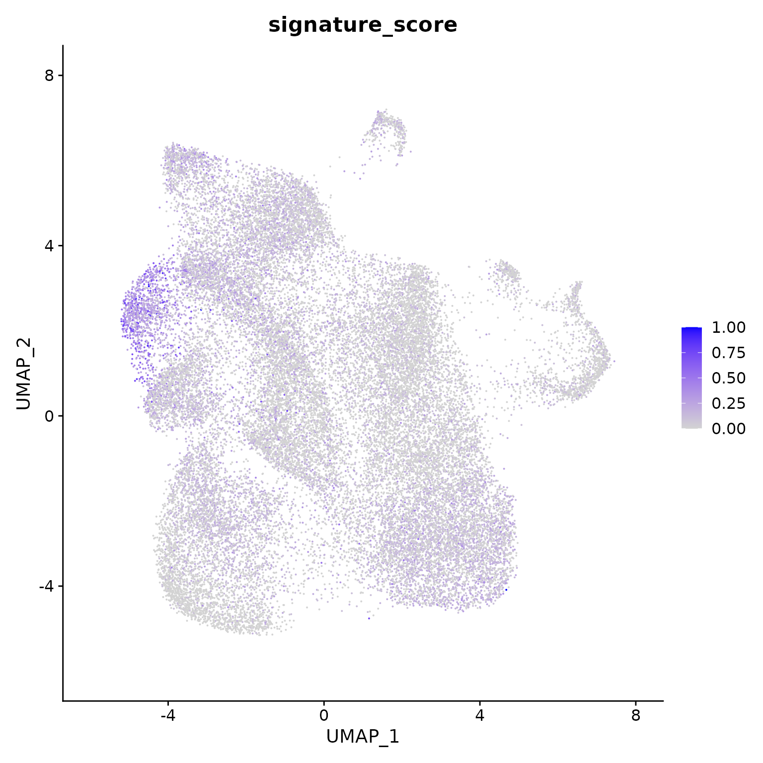

The cells could also be visualised using the popular and powerful ggplot package, enabling the researcher to use ggplot functions they were familiar with, and to customise the plot with great flexibility.

seurat_obj |>
    
    
    join_features(
        features = c("CD3D", "TRDC", "TRGC1", "TRGC2", "CD8A", "CD8B"),
        shape = "wide",
        assay = "SCT"
        
    ) |>
    
    mutate(signature_score =
                    scales::rescale(CD3D + TRDC + TRGC1+ TRGC2, to=c(0,1)) -
                    scales::rescale(CD8A + CD8B, to=c(0,1))
    ) |>
    
    # plot cells with high score last so they're not obscured by other cells
    arrange(signature_score) |>
    
    ggplot(aes(UMAP_1, UMAP_2, color = signature_score)) +
    geom_point(size=0.5) +
    scale_color_distiller(palette = "Spectral") +
    RMedicine2023tidytranscriptomics::theme_multipanel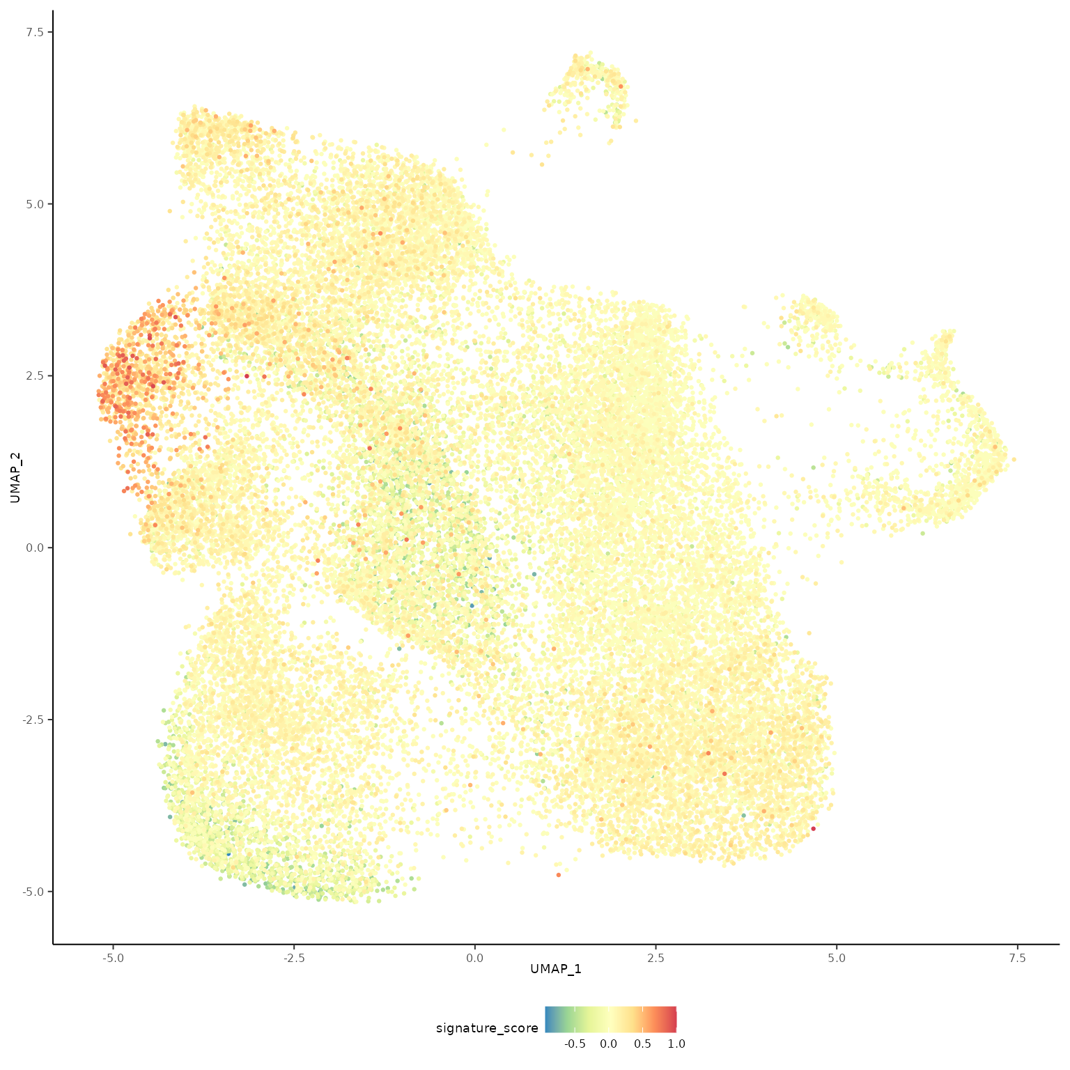

Filtering based on gate

The gamma delta T cells (the blue cluster on the left with high signature score) could be interactively selected from the plot using the tidygate package.

This code can only be executed interactively from an R file and not from a markdown file. So, in this casre, we need to copy and paste this into the console.

seurat_obj_gamma_delta = 
  seurat_obj |>
    
    
    join_features(
        features = c("CD3D", "TRDC", "TRGC1", "TRGC2", "CD8A", "CD8B"),
        shape = "wide",
        assay = "SCT"
        
    ) |>
    
    mutate(signature_score =
                    scales::rescale(CD3D + TRDC + TRGC1+ TRGC2, to=c(0,1)) -
                    scales::rescale(CD8A + CD8B, to=c(0,1))
    ) |>
    
    mutate(gate = tidygate::gate_int(
        UMAP_1, UMAP_2, 
        .size = 0.1, 
        .color =signature_score
    )) |> 
    
    filter(gate==1)

Filtering based on threshold

For exploratory analyses, we can select the gamma delta T cells, the red cluster on the left with high signature score. We’ll filter for cells with a signature score > 0.7.

seurat_obj_gamma_delta <-
    
    seurat_obj |>
    
    join_features(
        features = c("CD3D", "TRDC", "TRGC1", "TRGC2", "CD8A", "CD8B"), shape = "wide"
    ) |>
    
    mutate(
        signature_score =
            scales::rescale(CD3D + TRDC + TRGC1 + TRGC2, to = c(0, 1)) -
            scales::rescale(CD8A + CD8B, to = c(0, 1))
    ) |>
    
    # Proper cluster selection should be used instead (see supplementary material)
    filter(signature_score > 0.5)

Reanalysis after filtering

It was then possible to perform analyses on these gamma delta T cells by simply chaining further commands, such as below.

source("https://raw.githubusercontent.com/satijalab/seurat-wrappers/master/R/fast_mnn.R")

seurat_obj |>
    
    
    join_features(
        features = c("CD3D", "TRDC", "TRGC1", "TRGC2", "CD8A", "CD8B"),
        shape = "wide",
        assay = "SCT"
        
    ) |>
    
    mutate(signature_score =
                    scales::rescale(CD3D + TRDC + TRGC1+ TRGC2, to=c(0,1)) -
                    scales::rescale(CD8A + CD8B, to=c(0,1))
    ) |>
    
    # Proper cluster selection should be used instead (see supplementary material)
    filter(signature_score > 0.5) |> 
    
    # Reanalysis
    NormalizeData(assay="RNA") |> 
    FindVariableFeatures(nfeatures = 100, assay="RNA") |>
    SplitObject(split.by = "file") |> 
    SeuratWrappers::RunFastMNN(assay="RNA", features = 100) |> 
    RunUMAP(reduction = "mnn", dims = 1:20) |> 
    FindNeighbors(dims = 1:20, reduction = "mnn") |> 
    FindClusters(resolution = 0.3)

For comparison, we show the alternative using base R and SingleCellExperiment. Note that the code contains more redundancy and intermediate objects.

counts_positive <-
    assay(seurat_obj, "logcounts")[c("CD3D", "TRDC", "TRGC1", "TRGC2"), ] |>
    colSums() |>
    scales::rescale(to = c(0, 1))

counts_negative <-
    assay(seurat_obj, "logcounts")[c("CD8A", "CD8B"), ] |>
    colSums() |>
    scales::rescale(to = c(0, 1))

seurat_obj$signature_score <- counts_positive - counts_negative

seurat_obj_gamma_delta <- seurat_obj[, seurat_obj$signature_score > 0.7]

# Reanalysis
# ...

Interactive plotting

As a final note, it’s also possible to do complex and powerful things in a simple way, due to the integration of the tidy transcriptomics packages with the tidy universe. As one example, we can visualise the cells as a 3D plot using plotly.

The example data we’ve been using only contains a few genes, for the sake of time and size in this demonstration, but below is how you could generate the 3 dimensions needed for 3D plot with a full dataset.

single_cell_object |> 
    RunUMAP(dims = 1:30, n.components = 3L, spread = 0.5,min.dist  = 0.01, n.neighbors = 10L)

We’ll demonstrate creating a 3D plot using some data that has 3 UMAP dimensions.

seurat_obj_UMAP3 <- RMedicine2023tidytranscriptomics::seurat_obj_UMAP3

# Look at the object
seurat_obj_UMAP3 |> select(contains("UMAP"), everything())

## # A Seurat-tibble abstraction: 33,215 × 17
## # Features=1 | Cells=33215 | Active assay=integrated | Assays=integrated
##    .cell     file  Barcode batch BCB   S.Score G2M.Score Phase curated_cell_type
##    <chr>     <chr> <chr>   <chr> <chr>   <dbl>     <dbl> <chr> <chr>            
##  1 1_AAACGA… ../d… AAACGA… 1     BCB1…  0.0620   -0.0972 S     CD4+_Tcm_S100A4_…
##  2 1_AAACGC… ../d… AAACGC… 1     BCB1…  0.0943   -0.193  S     CD8+_high_ribonu…
##  3 1_AAACGC… ../d… AAACGC… 1     BCB1…  0.0216   -0.124  S     CD4+_Tcm_S100A4_…
##  4 1_AAAGAA… ../d… AAAGAA… 1     BCB1…  0.0598   -0.196  S     MAIT             
##  5 1_AAAGGA… ../d… AAAGGA… 1     BCB1…  0.0281   -0.0540 S     CD8+_high_ribonu…
##  6 1_AAAGGG… ../d… AAAGGG… 1     BCB1…  0.0110   -0.0998 S     MAIT             
##  7 1_AAAGGG… ../d… AAAGGG… 1     BCB1…  0.0341   -0.143  S     CD8+_high_ribonu…
##  8 1_AAAGTC… ../d… AAAGTC… 1     BCB1…  0.0425   -0.183  S     MAIT             
##  9 1_AAAGTC… ../d… AAAGTC… 1     BCB1… -0.0289   -0.127  G1    CD8+_high_ribonu…
## 10 1_AAAGTG… ../d… AAAGTG… 1     BCB1… -0.0551   -0.102  G1    CD8+_high_ribonu…
## # ℹ 33,205 more rows
## # ℹ 8 more variables: PC_1 <dbl>, PC_2 <dbl>, PC_3 <dbl>, PC_4 <dbl>,
## #   PC_5 <dbl>, UMAP_1 <dbl>, UMAP_2 <dbl>, UMAP_3 <dbl>

seurat_obj_UMAP3 |>
    
    tidyseurat::plot_ly(
        x = ~`UMAP_1`,
        y = ~`UMAP_2`,
        z = ~`UMAP_3`,
        color = ~curated_cell_type,
        colors = dittoSeq::dittoColors()
    ) |> 
    
    plotly::add_markers(size = I(1))

Exercises

What proportion of all cells are gamma-delta T cells?
There is a cluster of cells characterised by a low RNA output (nCount_RNA). Use tidygate to identify the cell composition (curated_cell_type) of that cluster.

Part 3 Nested analyses

When analysing single cell data is sometimes necessary to perform calculations on data subsets. For example, we might want to estimate difference in mRNA abundance between two condition for each cell type.

tidyr and purrr offer a great tool to perform iterativre analyses in a functional way.

We use tidyverse nest to group the data. The command below will create a tibble containing a column with a SummarizedExperiment object for each cell type. nest is similar to tidyverse group_by, except with nest each group is stored in a single row, and can be a complex object such as Seurat.

First let’s have a look to the cell types that constitute this dataset

seurat_obj |> 
  count(curated_cell_type)

## tidyseurat says: A data frame is returned for independent data analysis.

## # A tibble: 13 × 2
##    curated_cell_type                               n
##    <chr>                                       <int>
##  1 CD4+_Tcm_S100A4_IL32_IL7R_VIM                4978
##  2 CD8+_Tcm                                     3611
##  3 CD8+_Tem                                     4157
##  4 CD8+_high_ribonucleosome                     4885
##  5 CD8+_transitional_effector_GZMK_KLRB1_LYAR4  4138
##  6 HSC_lymphoid_myeloid_like                    1299
##  7 MAIT                                         1909
##  8 NK_cells                                     4535
##  9 NK_cycling                                    329
## 10 TCR_V_Delta_1                                 651
## 11 TCR_V_Delta_2                                 355
## 12 T_cell:CD8+_other                            2109
## 13 limphoid_myeloid_like_HLA_CD74                259

Let’s group the cells based on cell identity using nest

# Set idents for the differential analysis
Idents(seurat_obj) = seurat_obj[[]]$"treatment"

seurat_obj_nested = 
  seurat_obj |> 
  nest(seurat = -curated_cell_type) 

seurat_obj_nested

## # A tibble: 13 × 2
##    curated_cell_type                           seurat         
##    <chr>                                       <list>         
##  1 CD4+_Tcm_S100A4_IL32_IL7R_VIM               <Seurat[,4978]>
##  2 CD8+_high_ribonucleosome                    <Seurat[,4885]>
##  3 MAIT                                        <Seurat[,1909]>
##  4 CD8+_transitional_effector_GZMK_KLRB1_LYAR4 <Seurat[,4138]>
##  5 TCR_V_Delta_2                               <Seurat[,355]> 
##  6 T_cell:CD8+_other                           <Seurat[,2109]>
##  7 NK_cells                                    <Seurat[,4535]>
##  8 CD8+_Tem                                    <Seurat[,4157]>
##  9 CD8+_Tcm                                    <Seurat[,3611]>
## 10 TCR_V_Delta_1                               <Seurat[,651]> 
## 11 NK_cycling                                  <Seurat[,329]> 
## 12 HSC_lymphoid_myeloid_like                   <Seurat[,1299]>
## 13 limphoid_myeloid_like_HLA_CD74              <Seurat[,259]>

Let’s see what the first element of the Surat column looks like

seurat_obj_nested |> 
  slice(1) |> 
  pull(seurat)

## [[1]]
## # A Seurat-tibble abstraction: 4,978 × 17
## # Features=6 | Cells=4978 | Active assay=SCT | Assays=RNA, SCT
##    .cell     file  sample_id sample Barcode batch BCB    S.Score G2M.Score Phase
##    <chr>     <chr> <chr>     <chr>  <chr>   <chr> <chr>    <dbl>     <dbl> <chr>
##  1 1_AAACGA… ../d… SI-GA-H1… SI-GA… AAACGA… 1     BCB1…  0.0620   -0.0972  S    
##  2 1_AAACGC… ../d… SI-GA-H1… SI-GA… AAACGC… 1     BCB1…  0.0216   -0.124   S    
##  3 1_AAATGG… ../d… SI-GA-H1… SI-GA… AAATGG… 1     BCB1… -0.0195   -0.00881 G1   
##  4 1_AACAAA… ../d… SI-GA-H1… SI-GA… AACAAA… 1     BCB1…  0.0336   -0.147   S    
##  5 1_AACAAC… ../d… SI-GA-H1… SI-GA… AACAAC… 1     BCB1… -0.0421   -0.197   G1   
##  6 1_AACAAC… ../d… SI-GA-H1… SI-GA… AACAAC… 1     BCB1… -0.0105   -0.0902  G1   
##  7 1_AACACA… ../d… SI-GA-H1… SI-GA… AACACA… 1     BCB1…  0.00198  -0.0542  S    
##  8 1_AACCAA… ../d… SI-GA-H1… SI-GA… AACCAA… 1     BCB1… -0.00504  -0.135   G1   
##  9 1_AACCAA… ../d… SI-GA-H1… SI-GA… AACCAA… 1     BCB1…  0.0704   -0.145   S    
## 10 1_AACTTC… ../d… SI-GA-H1… SI-GA… AACTTC… 1     BCB1… -0.0336   -0.0956  G1   
## # ℹ 4,968 more rows
## # ℹ 7 more variables: nCount_RNA <dbl>, nFeature_RNA <int>, nCount_SCT <dbl>,
## #   nFeature_SCT <int>, treatment <fct>, UMAP_1 <dbl>, UMAP_2 <dbl>

Now, let’s perform a differential gene-transcript abundance analysis between the two conditions for each cell type.

seurat_obj_nested = 
  seurat_obj_nested |> 
  
  # Select significant genes
  mutate(significant_genes = map(
    seurat,
    ~ .x |> 
      
      # Test
      NormalizeData(assay="RNA") |> 
      FindAllMarkers(assay="RNA") |> 
      
      # Select top genes
      filter(p_val_adj<0.05) |> 
      head(10) |> 
      rownames()
  ))

seurat_obj_nested

## # A tibble: 13 × 3
##    curated_cell_type                           seurat          significant_genes
##    <chr>                                       <list>          <list>           
##  1 CD4+_Tcm_S100A4_IL32_IL7R_VIM               <Seurat[,4978]> <chr [10]>       
##  2 CD8+_high_ribonucleosome                    <Seurat[,4885]> <chr [10]>       
##  3 MAIT                                        <Seurat[,1909]> <chr [10]>       
##  4 CD8+_transitional_effector_GZMK_KLRB1_LYAR4 <Seurat[,4138]> <chr [10]>       
##  5 TCR_V_Delta_2                               <Seurat[,355]>  <chr [10]>       
##  6 T_cell:CD8+_other                           <Seurat[,2109]> <chr [10]>       
##  7 NK_cells                                    <Seurat[,4535]> <chr [10]>       
##  8 CD8+_Tem                                    <Seurat[,4157]> <chr [10]>       
##  9 CD8+_Tcm                                    <Seurat[,3611]> <chr [10]>       
## 10 TCR_V_Delta_1                               <Seurat[,651]>  <chr [10]>       
## 11 NK_cycling                                  <Seurat[,329]>  <chr [10]>       
## 12 HSC_lymphoid_myeloid_like                   <Seurat[,1299]> <chr [10]>       
## 13 limphoid_myeloid_like_HLA_CD74              <Seurat[,259]>  <chr [10]>

We can the lies the top genes with the heat map iteratively across the cell types

seurat_obj_nested = 
  seurat_obj_nested |> 
  
  # Build heatmaps
  mutate(heatmap = map2(
    seurat, significant_genes,
    ~ .x |> 
       ScaleData(assay="RNA") |> 
        DoHeatmap(.y, assay="RNA")
  )) 

seurat_obj_nested

## # A tibble: 13 × 4
##    curated_cell_type                seurat          significant_genes heatmap   
##    <chr>                            <list>          <list>            <list>    
##  1 CD4+_Tcm_S100A4_IL32_IL7R_VIM    <Seurat[,4978]> <chr [10]>        <patchwrk>
##  2 CD8+_high_ribonucleosome         <Seurat[,4885]> <chr [10]>        <patchwrk>
##  3 MAIT                             <Seurat[,1909]> <chr [10]>        <patchwrk>
##  4 CD8+_transitional_effector_GZMK… <Seurat[,4138]> <chr [10]>        <patchwrk>
##  5 TCR_V_Delta_2                    <Seurat[,355]>  <chr [10]>        <patchwrk>
##  6 T_cell:CD8+_other                <Seurat[,2109]> <chr [10]>        <patchwrk>
##  7 NK_cells                         <Seurat[,4535]> <chr [10]>        <patchwrk>
##  8 CD8+_Tem                         <Seurat[,4157]> <chr [10]>        <patchwrk>
##  9 CD8+_Tcm                         <Seurat[,3611]> <chr [10]>        <patchwrk>
## 10 TCR_V_Delta_1                    <Seurat[,651]>  <chr [10]>        <patchwrk>
## 11 NK_cycling                       <Seurat[,329]>  <chr [10]>        <patchwrk>
## 12 HSC_lymphoid_myeloid_like        <Seurat[,1299]> <chr [10]>        <patchwrk>
## 13 limphoid_myeloid_like_HLA_CD74   <Seurat[,259]>  <chr [10]>        <patchwrk>

Let’s have a look to the first heatmap

seurat_obj_nested |> 
  slice(1) |> 
  pull(heatmap)

## [[1]]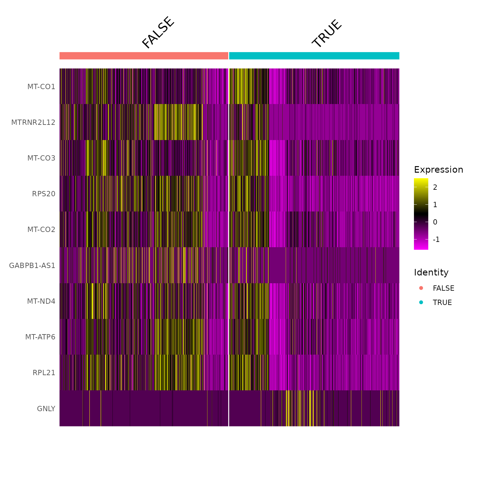

You can do this whole analysis without saving any temporary variable using the piping functionality of tidy R programming

seurat_obj |> 
  
  # Nest
  nest(seurat = -curated_cell_type) |> 
  
  # Select significant genes
  mutate(significant_genes = map(
    seurat,
    ~ .x |> 
      
      # Test
      NormalizeData(assay="RNA") |> 
      FindAllMarkers(assay="RNA") |> 
      
      # Select top genes
      filter(p_val_adj<0.05) |> 
      head(10) |> 
      rownames()
  )) |> 
  
  # Build heatmaps
  mutate(heatmap = map2(
    seurat, significant_genes,
    ~ .x |> 
       ScaleData(assay="RNA") |> 
        DoHeatmap(.y, assay="RNA")
  )) |> 
  
  # Extract heatmaps
  pull(heatmap)

Exercises

Let’s suppose that you want to perform the analyses only for cell types that have a total number of cells bigger than 1000. For example, if a cell type has less than a sum of 1000 cells across all samples, that cell type will be dropped from the dataset.

Answer this question avoiding to save temporary variables, and using the function add_count to count the cells (before nesting), and then filter
Answer this question avoiding to save temporary variables, and using the function map_int to count the cells (after nesting), and the filter

Part 4 Pseudobulk analyses

Next we want to identify genes whose transcription is affected by treatment in this dataset, comparing treated and untreated patients. We can do this with pseudobulk analysis. We aggregate cell-wise transcript abundance into pseudobulk samples and can then perform hypothesis testing using the very well established bulk RNA sequencing tools. For example, we can use DESeq2 in tidybulk to perform differential expression testing. For more details on pseudobulk analysis see here.

We want to do it for each cell type and the tidy transcriptomics ecosystem makes this very easy.

Create pseudobulk samples

To create pseudobulk samples from the single cell samples, we will use a helper function called aggregate_cells, available in this workshop package. This function will combine the single cells into a group for each cell type for each sample.

pseudo_bulk <-
    seurat_obj |>
    RMedicine2023tidytranscriptomics::aggregate_cells(c(sample, curated_cell_type), assays = "RNA")

pseudo_bulk

## # A SummarizedExperiment-tibble abstraction: 369,000 × 12
## # Features=3000 | Samples=123 | Assays=RNA
##    .feature .sample         RNA sample curated_cell_type .aggregated_cells file 
##    <chr>    <chr>         <dbl> <chr>  <chr>                         <int> <chr>
##  1 A1BG-AS1 SI-GA-E5___C…     1 SI-GA… CD4+_Tcm_S100A4_…               372 ../d…
##  2 A2M-AS1  SI-GA-E5___C…    14 SI-GA… CD4+_Tcm_S100A4_…               372 ../d…
##  3 AAED1    SI-GA-E5___C…    18 SI-GA… CD4+_Tcm_S100A4_…               372 ../d…
##  4 ABCA2    SI-GA-E5___C…     4 SI-GA… CD4+_Tcm_S100A4_…               372 ../d…
##  5 ABCB1    SI-GA-E5___C…    11 SI-GA… CD4+_Tcm_S100A4_…               372 ../d…
##  6 ABCC4    SI-GA-E5___C…     4 SI-GA… CD4+_Tcm_S100A4_…               372 ../d…
##  7 ABHD15   SI-GA-E5___C…     6 SI-GA… CD4+_Tcm_S100A4_…               372 ../d…
##  8 ABHD17A  SI-GA-E5___C…    50 SI-GA… CD4+_Tcm_S100A4_…               372 ../d…
##  9 ABHD17B  SI-GA-E5___C…     6 SI-GA… CD4+_Tcm_S100A4_…               372 ../d…
## 10 ABHD2    SI-GA-E5___C…    12 SI-GA… CD4+_Tcm_S100A4_…               372 ../d…
## # ℹ 40 more rows
## # ℹ 5 more variables: sample_id <chr>, batch <chr>, BCB <chr>, treatment <fct>,
## #   feature <chr>

Tidybulk and tidySummarizedExperiment

With tidySummarizedExperiment and tidybulk it is easy to split the data into groups and perform analyses on each without needing to create separate objects.

Tidybulk functions/utilities available

Function	Description
`aggregate_duplicates`	Aggregate abundance and annotation of duplicated transcripts in a robust way
`identify_abundant` `keep_abundant`	identify or keep the abundant genes
`keep_variable`	Filter for top variable features
`scale_abundance`	Scale (normalise) abundance for RNA sequencing depth
`reduce_dimensions`	Perform dimensionality reduction (PCA, MDS, tSNE, UMAP)
`cluster_elements`	Labels elements with cluster identity (kmeans, SNN)
`remove_redundancy`	Filter out elements with highly correlated features
`adjust_abundance`	Remove known unwanted variation (Combat)
`test_differential_abundance`	Differential transcript abundance testing (DESeq2, edgeR, voom)
`deconvolve_cellularity`	Estimated tissue composition (Cibersort, llsr, epic, xCell, mcp_counter, quantiseq
`test_differential_cellularity`	Differential cell-type abundance testing
`test_stratification_cellularity`	Estimate Kaplan-Meier survival differences
`test_gene_enrichment`	Gene enrichment analyses (EGSEA)
`test_gene_overrepresentation`	Gene enrichment on list of transcript names (no rank)
`test_gene_rank`	Gene enrichment on list of transcript (GSEA)
`impute_missing_abundance`	Impute abundance for missing data points using sample groupings

pseudo_bulk_nested <- 
    pseudo_bulk |>
    nest(grouped_summarized_experiment = -curated_cell_type)

pseudo_bulk_nested

## # A tibble: 13 × 2
##    curated_cell_type                           grouped_summarized_experiment
##    <chr>                                       <list>                       
##  1 CD4+_Tcm_S100A4_IL32_IL7R_VIM               <SmmrzdEx[,10]>              
##  2 CD8+_Tcm                                    <SmmrzdEx[,10]>              
##  3 CD8+_Tem                                    <SmmrzdEx[,10]>              
##  4 CD8+_high_ribonucleosome                    <SmmrzdEx[,10]>              
##  5 CD8+_transitional_effector_GZMK_KLRB1_LYAR4 <SmmrzdEx[,10]>              
##  6 HSC_lymphoid_myeloid_like                   <SmmrzdEx[,10]>              
##  7 MAIT                                        <SmmrzdEx[,10]>              
##  8 NK_cells                                    <SmmrzdEx[,10]>              
##  9 NK_cycling                                  <SmmrzdEx[,10]>              
## 10 TCR_V_Delta_1                               <SmmrzdEx[,10]>              
## 11 TCR_V_Delta_2                               <SmmrzdEx[,9]>               
## 12 T_cell:CD8+_other                           <SmmrzdEx[,10]>              
## 13 limphoid_myeloid_like_HLA_CD74              <SmmrzdEx[,4]>

To explore the grouping, we can use tidyverse slice to choose a row (cell_type) and pull to extract the values from a column. If we pull the data column we can view the SummarizedExperiment object.

pseudo_bulk_nested |>
    slice(1) |>
    pull(grouped_summarized_experiment)

## [[1]]
## # A SummarizedExperiment-tibble abstraction: 30,000 × 11
## # Features=3000 | Samples=10 | Assays=RNA
##    .feature .sample     RNA sample .aggregated_cells file  sample_id batch BCB  
##    <chr>    <chr>     <dbl> <chr>              <int> <chr> <chr>     <chr> <chr>
##  1 A1BG-AS1 SI-GA-E5…     1 SI-GA…               372 ../d… SI-GA-E5… 2     BCB0…
##  2 A2M-AS1  SI-GA-E5…    14 SI-GA…               372 ../d… SI-GA-E5… 2     BCB0…
##  3 AAED1    SI-GA-E5…    18 SI-GA…               372 ../d… SI-GA-E5… 2     BCB0…
##  4 ABCA2    SI-GA-E5…     4 SI-GA…               372 ../d… SI-GA-E5… 2     BCB0…
##  5 ABCB1    SI-GA-E5…    11 SI-GA…               372 ../d… SI-GA-E5… 2     BCB0…
##  6 ABCC4    SI-GA-E5…     4 SI-GA…               372 ../d… SI-GA-E5… 2     BCB0…
##  7 ABHD15   SI-GA-E5…     6 SI-GA…               372 ../d… SI-GA-E5… 2     BCB0…
##  8 ABHD17A  SI-GA-E5…    50 SI-GA…               372 ../d… SI-GA-E5… 2     BCB0…
##  9 ABHD17B  SI-GA-E5…     6 SI-GA…               372 ../d… SI-GA-E5… 2     BCB0…
## 10 ABHD2    SI-GA-E5…    12 SI-GA…               372 ../d… SI-GA-E5… 2     BCB0…
## # ℹ 40 more rows
## # ℹ 2 more variables: treatment <fct>, feature <chr>

We can then identify differentially expressed genes for each cell type for our condition of interest, treated versus untreated patients. We use tidyverse map to apply differential expression functions to each cell type group in the nested data. The result columns will be added to the SummarizedExperiment objects.

# Differential transcription abundance
pseudo_bulk_nested <-
    
    pseudo_bulk_nested |>
    
    # map accepts a data column (.x) and a function. It applies the function to each element of the column.
    mutate(grouped_summarized_experiment = map(
        grouped_summarized_experiment,
        ~ .x |>
            
            # Removing genes with low expression
            keep_abundant(factor_of_interest = treatment) |>
            
            # Testing for differential expression using DESeq2  
            test_differential_abundance(~treatment, method="DESeq2") |> 
            
            # Scale abundance for FUTURE visualisation
            scale_abundance(method="TMMwsp") 
    ))

The output is again a tibble containing a SummarizedExperiment object for each cell type.

pseudo_bulk_nested

## # A tibble: 13 × 2
##    curated_cell_type                           grouped_summarized_experiment
##    <chr>                                       <list>                       
##  1 CD4+_Tcm_S100A4_IL32_IL7R_VIM               <SmmrzdEx[,10]>              
##  2 CD8+_Tcm                                    <SmmrzdEx[,10]>              
##  3 CD8+_Tem                                    <SmmrzdEx[,10]>              
##  4 CD8+_high_ribonucleosome                    <SmmrzdEx[,10]>              
##  5 CD8+_transitional_effector_GZMK_KLRB1_LYAR4 <SmmrzdEx[,10]>              
##  6 HSC_lymphoid_myeloid_like                   <SmmrzdEx[,10]>              
##  7 MAIT                                        <SmmrzdEx[,10]>              
##  8 NK_cells                                    <SmmrzdEx[,10]>              
##  9 NK_cycling                                  <SmmrzdEx[,10]>              
## 10 TCR_V_Delta_1                               <SmmrzdEx[,10]>              
## 11 TCR_V_Delta_2                               <SmmrzdEx[,9]>               
## 12 T_cell:CD8+_other                           <SmmrzdEx[,10]>              
## 13 limphoid_myeloid_like_HLA_CD74              <SmmrzdEx[,4]>

If we pull out the SummarizedExperiment object for the first cell type, as before, we can see it now has columns containing the differential expression results (e.g. logFC, PValue).

pseudo_bulk_nested |>
    slice(1) |>
    pull(grouped_summarized_experiment)

## [[1]]
## # A SummarizedExperiment-tibble abstraction: 14,580 × 21
## # Features=1458 | Samples=10 | Assays=RNA, RNA_scaled
##    .feature .sample      RNA RNA_scaled sample .aggregated_cells file  sample_id
##    <chr>    <chr>      <dbl>      <dbl> <chr>              <int> <chr> <chr>    
##  1 A2M-AS1  SI-GA-E5_…    14       56.3 SI-GA…               372 ../d… SI-GA-E5…
##  2 AAED1    SI-GA-E5_…    18       72.4 SI-GA…               372 ../d… SI-GA-E5…
##  3 ABCA2    SI-GA-E5_…     4       16.1 SI-GA…               372 ../d… SI-GA-E5…
##  4 ABCB1    SI-GA-E5_…    11       44.2 SI-GA…               372 ../d… SI-GA-E5…
##  5 ABHD15   SI-GA-E5_…     6       24.1 SI-GA…               372 ../d… SI-GA-E5…
##  6 ABHD17A  SI-GA-E5_…    50      201.  SI-GA…               372 ../d… SI-GA-E5…
##  7 ABHD17B  SI-GA-E5_…     6       24.1 SI-GA…               372 ../d… SI-GA-E5…
##  8 ABHD2    SI-GA-E5_…    12       48.3 SI-GA…               372 ../d… SI-GA-E5…
##  9 ABHD5    SI-GA-E5_…     5       20.1 SI-GA…               372 ../d… SI-GA-E5…
## 10 ABI2     SI-GA-E5_…    22       88.5 SI-GA…               372 ../d… SI-GA-E5…
## # ℹ 40 more rows
## # ℹ 13 more variables: batch <chr>, BCB <chr>, treatment <fct>, TMM <dbl>,
## #   multiplier <dbl>, feature <chr>, .abundant <lgl>, baseMean <dbl>,
## #   log2FoldChange <dbl>, lfcSE <dbl>, stat <dbl>, pvalue <dbl>, padj <dbl>

We can analyse our nested dataset mapping queries across the SummarizedExperiments

pseudo_bulk_nested = 
    pseudo_bulk_nested |>
    
    # Identify top significant genes
    mutate(top_genes = map_chr(
        grouped_summarized_experiment, 
        ~ .x |> 
            pivot_transcript() |> 
            arrange(pvalue) |> 
            head(1) |> 
            pull(.feature)
    )) |> 
    
    # Filter top gene
    mutate(grouped_summarized_experiment = map2(
        grouped_summarized_experiment, top_genes,
        ~ filter(.x, .feature == .y)
    )) 

pseudo_bulk_nested

## # A tibble: 13 × 3
##    curated_cell_type                           grouped_summarized_ex…¹ top_genes
##    <chr>                                       <list>                  <chr>    
##  1 CD4+_Tcm_S100A4_IL32_IL7R_VIM               <SmmrzdEx[,10]>         MIAT     
##  2 CD8+_Tcm                                    <SmmrzdEx[,10]>         SH3BGRL3 
##  3 CD8+_Tem                                    <SmmrzdEx[,10]>         MT-CO1   
##  4 CD8+_high_ribonucleosome                    <SmmrzdEx[,10]>         PPBP     
##  5 CD8+_transitional_effector_GZMK_KLRB1_LYAR4 <SmmrzdEx[,10]>         TYROBP   
##  6 HSC_lymphoid_myeloid_like                   <SmmrzdEx[,10]>         GABPB1-A…
##  7 MAIT                                        <SmmrzdEx[,10]>         MT-CO1   
##  8 NK_cells                                    <SmmrzdEx[,10]>         MT-CO1   
##  9 NK_cycling                                  <SmmrzdEx[,10]>         CD3G     
## 10 TCR_V_Delta_1                               <SmmrzdEx[,10]>         PRF1     
## 11 TCR_V_Delta_2                               <SmmrzdEx[,9]>          MT-CO1   
## 12 T_cell:CD8+_other                           <SmmrzdEx[,10]>         CTSW     
## 13 limphoid_myeloid_like_HLA_CD74              <SmmrzdEx[,4]>          GNLY     
## # ℹ abbreviated name: ¹grouped_summarized_experiment

Plot top differential genes

pseudo_bulk_nested = 
    pseudo_bulk_nested |>
    
    # Plot significant genes for each cell type
    # map2 is map that accepts 2 input columns (.x, .y) and a function
    mutate(plot = map2(
        grouped_summarized_experiment,curated_cell_type,
        ~ .x |>
            
            # Plot
            ggplot(aes(treatment, RNA_scaled + 1)) +
            geom_boxplot(aes(fill = treatment)) +
            geom_jitter() +
            scale_y_log10() +
            facet_wrap(~.feature, ncol = 3) +
            ggtitle(.y) +
            RMedicine2023tidytranscriptomics::theme_multipanel
    )) 

pseudo_bulk_nested

## # A tibble: 13 × 4
##    curated_cell_type                      grouped_summarized_e…¹ top_genes plot 
##    <chr>                                  <list>                 <chr>     <lis>
##  1 CD4+_Tcm_S100A4_IL32_IL7R_VIM          <SmmrzdEx[,10]>        MIAT      <gg> 
##  2 CD8+_Tcm                               <SmmrzdEx[,10]>        SH3BGRL3  <gg> 
##  3 CD8+_Tem                               <SmmrzdEx[,10]>        MT-CO1    <gg> 
##  4 CD8+_high_ribonucleosome               <SmmrzdEx[,10]>        PPBP      <gg> 
##  5 CD8+_transitional_effector_GZMK_KLRB1… <SmmrzdEx[,10]>        TYROBP    <gg> 
##  6 HSC_lymphoid_myeloid_like              <SmmrzdEx[,10]>        GABPB1-A… <gg> 
##  7 MAIT                                   <SmmrzdEx[,10]>        MT-CO1    <gg> 
##  8 NK_cells                               <SmmrzdEx[,10]>        MT-CO1    <gg> 
##  9 NK_cycling                             <SmmrzdEx[,10]>        CD3G      <gg> 
## 10 TCR_V_Delta_1                          <SmmrzdEx[,10]>        PRF1      <gg> 
## 11 TCR_V_Delta_2                          <SmmrzdEx[,9]>         MT-CO1    <gg> 
## 12 T_cell:CD8+_other                      <SmmrzdEx[,10]>        CTSW      <gg> 
## 13 limphoid_myeloid_like_HLA_CD74         <SmmrzdEx[,4]>         GNLY      <gg> 
## # ℹ abbreviated name: ¹grouped_summarized_experiment

pseudo_bulk_nested |> pull(plot)

## [[1]]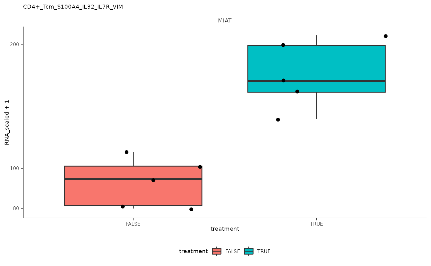

## 
## [[2]]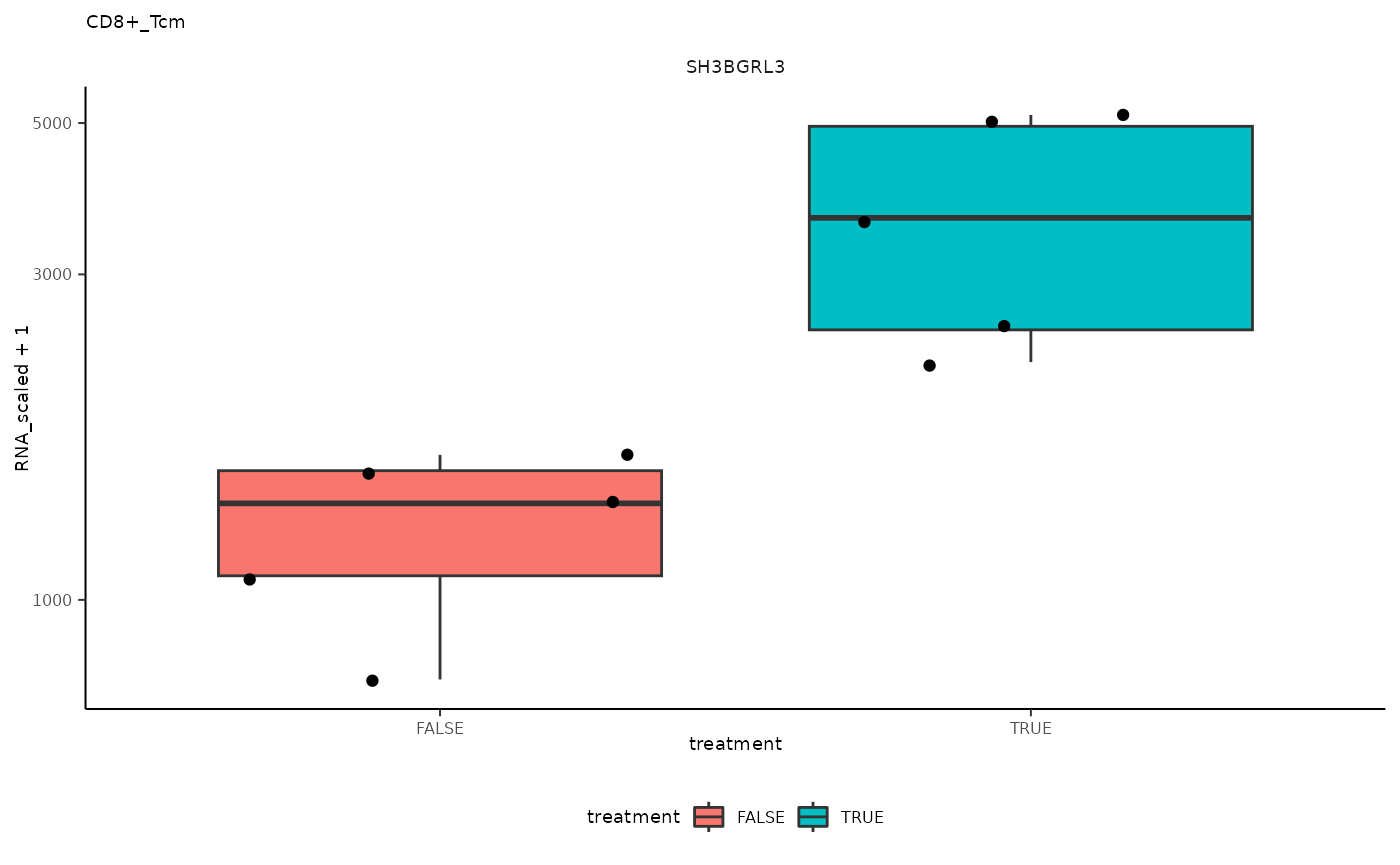

## 
## [[3]]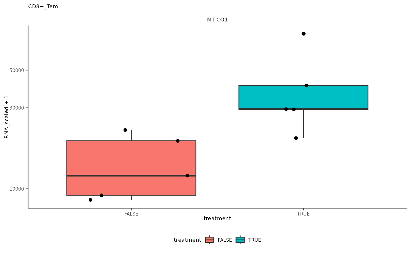

## 
## [[4]]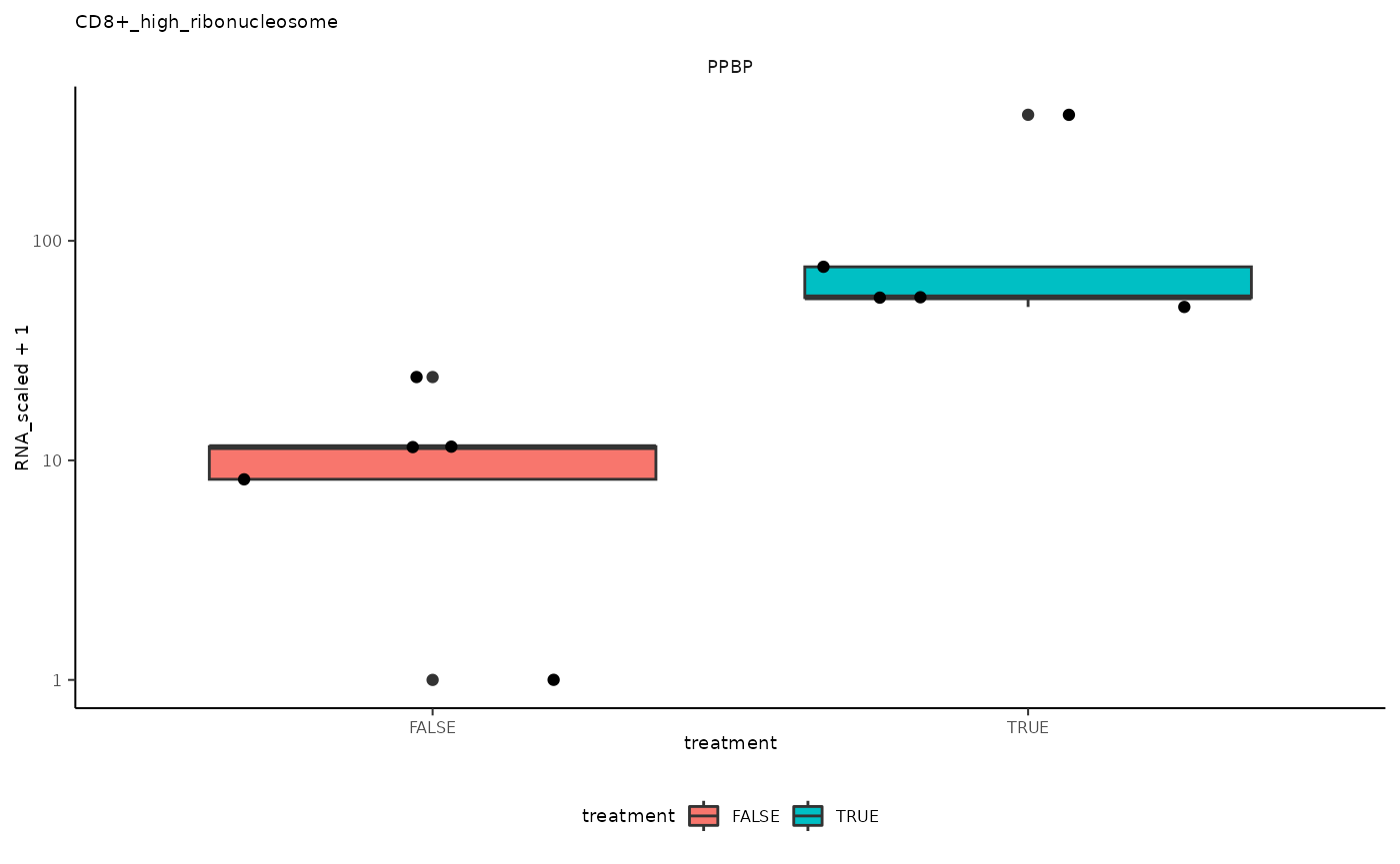

## 
## [[5]]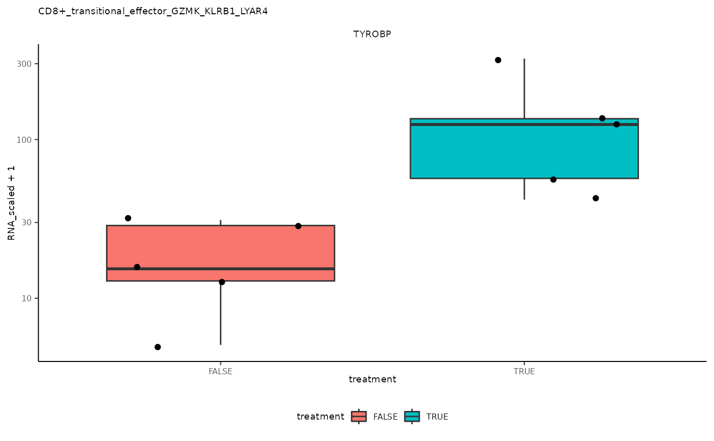

## 
## [[6]]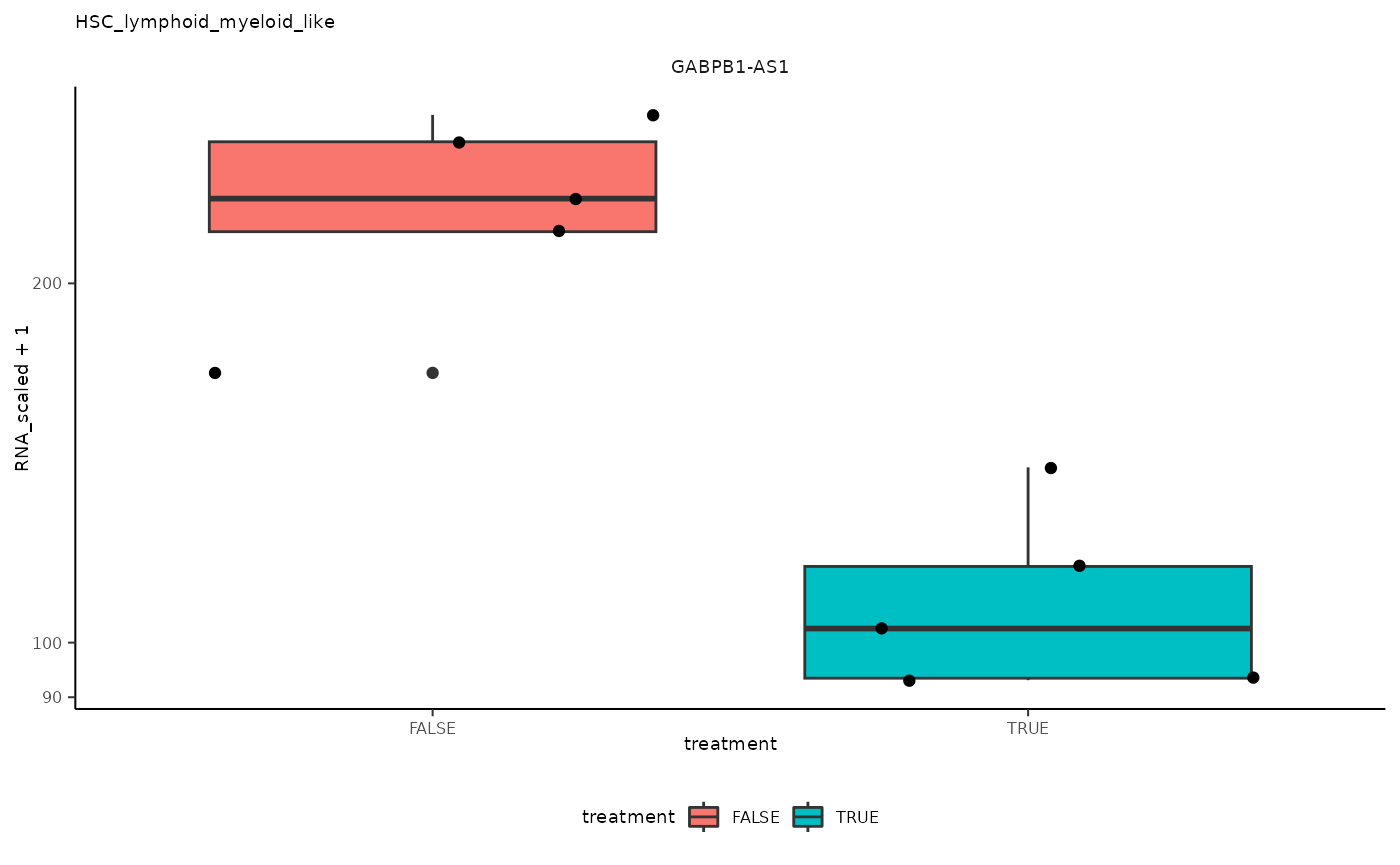

## 
## [[7]]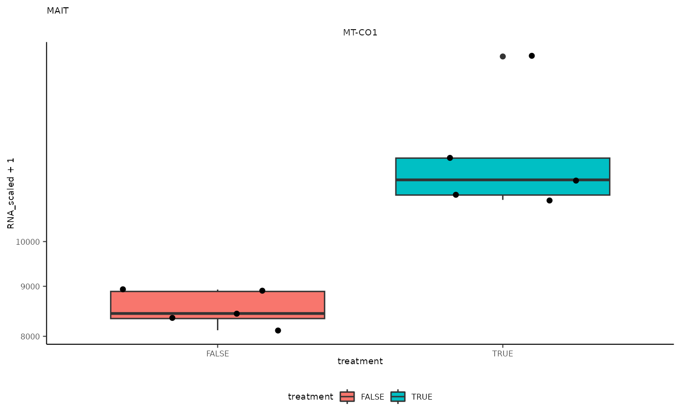

## 
## [[8]]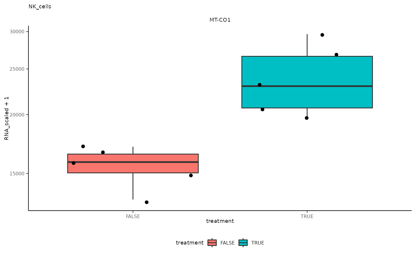

## 
## [[9]]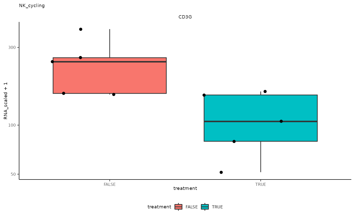

## 
## [[10]]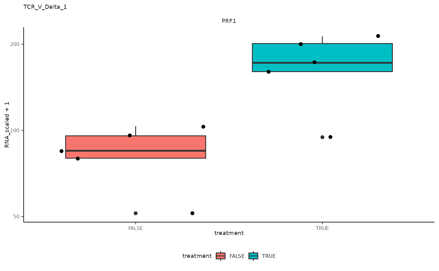

## 
## [[11]]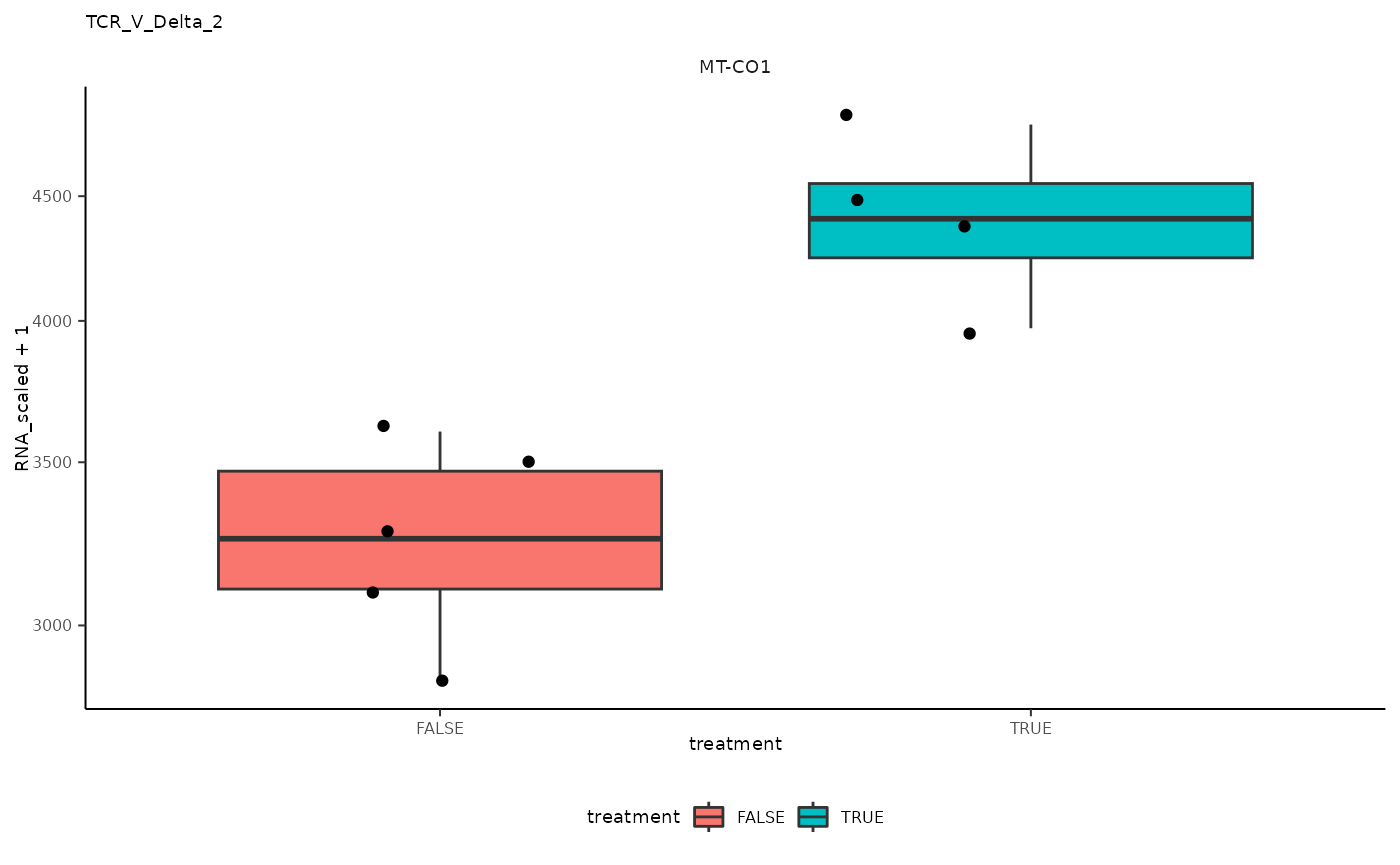

## 
## [[12]]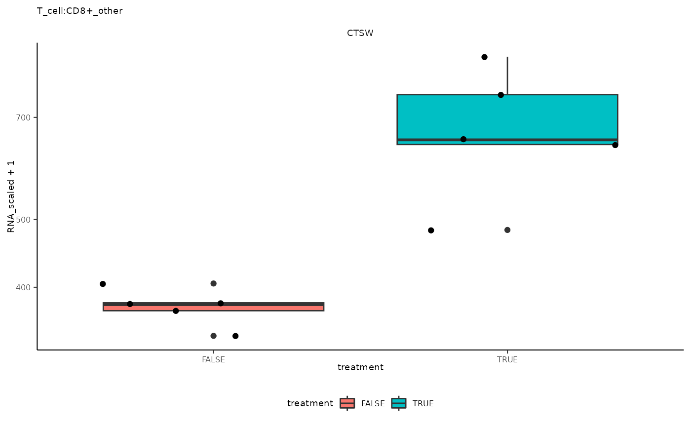

## 
## [[13]]

Session Information

sessionInfo()

## R version 4.2.1 (2022-06-23)
## Platform: x86_64-pc-linux-gnu (64-bit)
## Running under: Ubuntu 20.04.4 LTS
## 
## Matrix products: default
## BLAS:   /usr/lib/x86_64-linux-gnu/openblas-pthread/libblas.so.3
## LAPACK: /usr/lib/x86_64-linux-gnu/openblas-pthread/liblapack.so.3
## 
## locale:
##  [1] LC_CTYPE=en_US.UTF-8       LC_NUMERIC=C              
##  [3] LC_TIME=en_US.UTF-8        LC_COLLATE=en_US.UTF-8    
##  [5] LC_MONETARY=en_US.UTF-8    LC_MESSAGES=en_US.UTF-8   
##  [7] LC_PAPER=en_US.UTF-8       LC_NAME=C                 
##  [9] LC_ADDRESS=C               LC_TELEPHONE=C            
## [11] LC_MEASUREMENT=en_US.UTF-8 LC_IDENTIFICATION=C       
## 
## attached base packages:
## [1] stats4    stats     graphics  grDevices utils     datasets  methods  
## [8] base     
## 
## other attached packages:
##  [1] tidySummarizedExperiment_1.9.1 SummarizedExperiment_1.26.1   
##  [3] Biobase_2.56.0                 GenomicRanges_1.48.0          
##  [5] GenomeInfoDb_1.32.4            IRanges_2.30.1                
##  [7] S4Vectors_0.34.0               BiocGenerics_0.42.0           
##  [9] MatrixGenerics_1.8.1           matrixStats_1.0.0             
## [11] tidybulk_1.11.1                tidyr_1.3.0                   
## [13] glue_1.6.2                     tidyseurat_0.5.9              
## [15] ttservice_0.3.5                dittoSeq_1.8.1                
## [17] colorspace_2.1-0               dplyr_1.1.2                   
## [19] ggplot2_3.4.2                  SeuratObject_4.1.3            
## [21] Seurat_4.3.0                   purrr_1.0.1                   
## 
## loaded via a namespace (and not attached):
##   [1] utf8_1.2.3                             
##   [2] spatstat.explore_3.2-1                 
##   [3] reticulate_1.29                        
##   [4] tidyselect_1.2.0                       
##   [5] RSQLite_2.3.1                          
##   [6] AnnotationDbi_1.58.0                   
##   [7] htmlwidgets_1.6.2                      
##   [8] grid_4.2.1                             
##   [9] BiocParallel_1.30.4                    
##  [10] Rtsne_0.16                             
##  [11] munsell_0.5.0                          
##  [12] codetools_0.2-19                       
##  [13] ragg_1.2.5                             
##  [14] ica_1.0-3                              
##  [15] preprocessCore_1.58.0                  
##  [16] future_1.32.0                          
##  [17] miniUI_0.1.1.1                         
##  [18] withr_2.5.0                            
##  [19] spatstat.random_3.1-5                  
##  [20] progressr_0.13.0                       
##  [21] highr_0.10                             
##  [22] knitr_1.43                             
##  [23] SingleCellExperiment_1.18.1            
##  [24] ROCR_1.0-11                            
##  [25] tensor_1.5                             
##  [26] listenv_0.9.0                          
##  [27] labeling_0.4.2                         
##  [28] GenomeInfoDbData_1.2.8                 
##  [29] polyclip_1.10-4                        
##  [30] bit64_4.0.5                            
##  [31] farver_2.1.1                           
##  [32] pheatmap_1.0.12                        
##  [33] rprojroot_2.0.3                        
##  [34] parallelly_1.36.0                      
##  [35] vctrs_0.6.2                            
##  [36] generics_0.1.3                         
##  [37] xfun_0.39                              
##  [38] R6_2.5.1                               
##  [39] locfit_1.5-9.7                         
##  [40] bitops_1.0-7                           
##  [41] spatstat.utils_3.0-3                   
##  [42] cachem_1.0.8                           
##  [43] DelayedArray_0.22.0                    
##  [44] promises_1.2.0.1                       
##  [45] scales_1.2.1                           
##  [46] gtable_0.3.3                           
##  [47] RMedicine2023tidytranscriptomics_0.15.0
##  [48] globals_0.16.2                         
##  [49] goftest_1.2-3                          
##  [50] rlang_1.1.1                            
##  [51] genefilter_1.78.0                      
##  [52] systemfonts_1.0.4                      
##  [53] splines_4.2.1                          
##  [54] lazyeval_0.2.2                         
##  [55] spatstat.geom_3.2-1                    
##  [56] BiocManager_1.30.20                    
##  [57] yaml_2.3.7                             
##  [58] reshape2_1.4.4                         
##  [59] abind_1.4-5                            
##  [60] crosstalk_1.2.0                        
##  [61] httpuv_1.6.11                          
##  [62] tools_4.2.1                            
##  [63] ellipsis_0.3.2                         
##  [64] jquerylib_0.1.4                        
##  [65] RColorBrewer_1.1-3                     
##  [66] ggridges_0.5.4                         
##  [67] Rcpp_1.0.10                            
##  [68] plyr_1.8.8                             
##  [69] zlibbioc_1.42.0                        
##  [70] RCurl_1.98-1.12                        
##  [71] deldir_1.0-9                           
##  [72] pbapply_1.7-0                          
##  [73] cowplot_1.1.1                          
##  [74] zoo_1.8-12                             
##  [75] ggrepel_0.9.3                          
##  [76] cluster_2.1.4                          
##  [77] fs_1.6.2                               
##  [78] magrittr_2.0.3                         
##  [79] data.table_1.14.8                      
##  [80] scattermore_1.1                        
##  [81] lmtest_0.9-40                          
##  [82] RANN_2.6.1                             
##  [83] fitdistrplus_1.1-11                    
##  [84] hms_1.1.3                              
##  [85] patchwork_1.1.2                        
##  [86] mime_0.12                              
##  [87] evaluate_0.21                          
##  [88] xtable_1.8-4                           
##  [89] XML_3.99-0.14                          
##  [90] gridExtra_2.3                          
##  [91] compiler_4.2.1                         
##  [92] tibble_3.2.1                           
##  [93] crayon_1.5.2                           
##  [94] KernSmooth_2.23-21                     
##  [95] htmltools_0.5.5                        
##  [96] later_1.3.1                            
##  [97] tzdb_0.4.0                             
##  [98] geneplotter_1.74.0                     
##  [99] DBI_1.1.3                              
## [100] MASS_7.3-60                            
## [101] Matrix_1.5-4.1                         
## [102] readr_2.1.4                            
## [103] cli_3.6.1                              
## [104] parallel_4.2.1                         
## [105] igraph_1.4.3                           
## [106] pkgconfig_2.0.3                        
## [107] pkgdown_2.0.7                          
## [108] sp_1.6-1                               
## [109] plotly_4.10.2                          
## [110] spatstat.sparse_3.0-1                  
## [111] annotate_1.74.0                        
## [112] bslib_0.4.2                            
## [113] XVector_0.36.0                         
## [114] stringr_1.5.0                          
## [115] digest_0.6.31                          
## [116] sctransform_0.3.5                      
## [117] RcppAnnoy_0.0.20                       
## [118] Biostrings_2.64.1                      
## [119] spatstat.data_3.0-1                    
## [120] rmarkdown_2.22                         
## [121] leiden_0.4.3                           
## [122] uwot_0.1.14                            
## [123] edgeR_3.38.4                           
## [124] shiny_1.7.4                            
## [125] lifecycle_1.0.3                        
## [126] nlme_3.1-162                           
## [127] jsonlite_1.8.5                         
## [128] desc_1.4.2                             
## [129] viridisLite_0.4.2                      
## [130] limma_3.52.4                           
## [131] fansi_1.0.4                            
## [132] pillar_1.9.0                           
## [133] lattice_0.21-8                         
## [134] KEGGREST_1.36.3                        
## [135] fastmap_1.1.1                          
## [136] httr_1.4.6                             
## [137] survival_3.5-5                         
## [138] png_0.1-8                              
## [139] bit_4.0.5                              
## [140] stringi_1.7.12                         
## [141] sass_0.4.6                             
## [142] blob_1.2.4                             
## [143] textshaping_0.3.6                      
## [144] DESeq2_1.36.0                          
## [145] memoise_2.0.1                          
## [146] irlba_2.3.5.1                          
## [147] future.apply_1.11.0

References

Butler, Andrew, Paul Hoffman, Peter Smibert, Efthymia Papalexi, and Rahul Satija. 2018. “Integrating Single-Cell Transcriptomic Data Across Different Conditions, Technologies, and Species.” Nature Biotechnology 36 (5): 411–20.

Pizzolato, Gabriele, Hannah Kaminski, Marie Tosolini, Don-Marc Franchini, Fréderic Pont, Fréderic Martins, Carine Valle, et al. 2019. “Single-Cell RNA Sequencing Unveils the Shared and the Distinct Cytotoxic Hallmarks of Human TCRV\(\updelta\)1 and TCRV\(\updelta\)2 \(\upgamma\)\(\updelta\) t Lymphocytes.” Proceedings of the National Academy of Sciences, May, 201818488. https://doi.org/10.1073/pnas.1818488116.

Stuart, Tim, Andrew Butler, Paul Hoffman, Christoph Hafemeister, Efthymia Papalexi, William M Mauck III, Yuhan Hao, Marlon Stoeckius, Peter Smibert, and Rahul Satija. 2019. “Comprehensive Integration of Single-Cell Data.” Cell 177 (7): 1888–1902.

Wickham, Hadley, Mara Averick, Jennifer Bryan, Winston Chang, Lucy D’Agostino McGowan, Romain François, Garrett Grolemund, et al. 2019. “Welcome to the Tidyverse.” Journal of Open Source Software 4 (43): 1686.

<maria.doyle at petermac.org>↩︎
<mangiola.s at wehi.edu.au>↩︎

Maria Doyle, Peter MacCallum Cancer Centre¹

Stefano Mangiola, Walter and Eliza Hall Institute²

Instructors

Workshop goals and objectives

What you will learn

What you will not learn

Getting started

Local

Introduction to tidytranscriptomics

Part 1 Introduction to tidyseurat

Tidyverse commands

Part 2 Signature visualisation

Data pre-processing

Analyse custom signature

Signature calculation

Filtering based on gate

Filtering based on threshold

Reanalysis after filtering

Interactive plotting

Exercises

Part 3 Nested analyses

Exercises

Part 4 Pseudobulk analyses

Create pseudobulk samples

Tidybulk and tidySummarizedExperiment

Tidybulk functions/utilities available

Tidy Transcriptomics for Single-cell RNA Sequencing Analyses

Maria Doyle, Peter MacCallum Cancer Centre1

Stefano Mangiola, Walter and Eliza Hall Institute2

Instructors

Workshop goals and objectives

What you will learn

What you will not learn

Getting started

Local

Introduction to tidytranscriptomics

Part 1 Introduction to tidyseurat

Tidyverse commands

Part 2 Signature visualisation

Data pre-processing

Analyse custom signature

Signature calculation

Filtering based on gate

Filtering based on threshold

Reanalysis after filtering

Interactive plotting

Exercises

Part 3 Nested analyses

Exercises

Part 4 Pseudobulk analyses

Create pseudobulk samples

Tidybulk and tidySummarizedExperiment

Tidybulk functions/utilities available

Maria Doyle, Peter MacCallum Cancer Centre¹

Stefano Mangiola, Walter and Eliza Hall Institute²